1. Introduction

The origin of dark matter (DM) remains one of the greatest mysteries in modern Physics [1]. So far, we have detected only the gravitational effects of DM from different astrophysical sources, from galaxy clusters to single galaxies. The observed evidence of DM can be explained with at least one new particle with respect to the Standard Model. Despite the overwhelming gravitational evidence, no conclusive detection has been done on its particle properties. Therefore, the properties of DM are still not completely understood today. We know that DM constitutes up to 85% of the Universe’s matter and, if made of particles, it is massive and non-relativistic in the current Universe, and non-baryonic and stable on cosmological scales. DM is very weakly interacting, that is, it does not emit, absorb, or reflect light. Thus, it is very difficult to detect using traditional methods. Although we do not know the true nature of DM, its existence can be proven to account for observations in several astrophysical objects from cluster of galaxies up to individual galaxies.

The first historical evidence of DM was achieved by measuring the mass of galaxies. The mass of a galaxy can be measured using two methods. First, its luminosity through the flux emitted by stars: the brighter an object, the more massive it is. Second, the velocities of stars present in the galaxy. In particular, the virial theorem can be used to calculate the gravitational mass, which is the real total mass connected to the gravitational force. In the early 20th century, a Swiss astronomy professor Fritz Zwicky was observing the Coma cluster and he realized that the luminous mass and the gravitational mass of the cluster did not match. The galaxies in the cluster were moving way too rapidly - about 100 times faster than expected for luminous matter, as the luminous mass was only about a few percent of the gravitational mass. Zwicky concluded that the "missing" matter was really present, but we could not see it because it is of non-baryonic matter. This was the beginning of what he coined dunkle materie, or dark matter.

One of the most precise pieces of evidence of DM is related to the rotational velocities of stars in galaxies. The American astronomer Vera Rubin's discoveries were monumental in the establishment of the distribution of DM. According to Kepler's laws, the rotational velocity v of an object at a radius r away from the center of orbit should be:

\( v= \frac{\sqrt[]{GM(r)}}{r} \) (1)

where G is the gravitational constant and M(r) is the mass of the Galaxy for radii smaller than r. Farther away from the center, the increasing radius should cause the rotation velocities of objects such as stars and gases to decrease (specifically, when written as a function of radius r, at a rate of \( \frac{1}{\sqrt[]{r}} \) ). This implies that the velocity graph should look like the line labeled "disk" in figure 1, where we show the data of the rotational velocity for the galaxy NGC 3198 together with the theoretical predictions for different components. However, the data for the velocity rotation curve of the galaxy stays constant even as the radius increases. To account for this discrepancy, a new matter component which creates an increasing velocity for large radii should be present.

Known types of matter (i.e. baryonic matter) at the time could not explain the phenomenon. Therefore, scientists decided that a new type of invisible particle - DM - was contributing to the constant mass at the edges of the galaxy. In particular, using the flatness of the rotational velocity data, we can estimate that DM should be present with a spherical halo around galaxies that extends up to 100-200 kpc from the center with a radial dependence of the order of \( ρ∝{r^{-2}} \) .

Today, we call it the DM halo. The density of the DM halo, in particular, is of great interest to the astrophysical community.

Figure 1. This figure represents the profile of the rotational velocity in the galaxy NGC 3198, which is due to the disk and the DM halo. This figure is taken from [2].

2. DM profiles

To calculate the DM density, we use a variety of DM profiles: Navarro-Frenk-White (NFW), Einasto, Isothermal, Burkert, and Moore. Each model is justified by observations of specific astrophysical objects from N-body simulations. N-body simulations typically give cusp profiles such as NFW and Einasto, while the observations of galaxies and dwarf planets can be explained with core density profiles such as Burkert or Isothermal. It is thus beneficial to consider all of them. NFW is the traditional choice and Einasto seems to fit more recent simulations with a parameter \( α \) which we will set to 0.17 in this experiment. Isothermal and Burkert are more motivated by velocity rotation curves but seem to conflict with recent simulations, while Moore provides a profile steeper than NFW. As functions \( ρ(r) \) ,where r is the radius, they are written as:

NFW: \( ρ(r)={ρ_{s}}\frac{{r_{s}}}{r}{(1+\frac{r}{{r_{s}}})^{-2}} \)

Einasto: \( ρ(r)={ρ_{s}}exp\lbrace -\frac{2}{α}[{(\frac{r}{{r_{s}}})^{α}}-1]\rbrace \)

Isothermal: \( ρ(r)=\frac{{ρ_{s}}}{1+{(r/{r_{s}})^{2}}} \) (2)

Burkert: \( ρ(r)=\frac{{ρ_{s}}}{(1+r/{r_{s}})(1+{(r/{r_{s}})^{2}})} \)

Moore: \( ρ(r)={ρ_{s}}{(\frac{{r_{s}}}{r})^{1.16}}{(1+\frac{r}{{r_{s}}})^{-1.84}} \)

The existence of baryons can modify the slope of the DM density profiles. In particular, for cusp profiles, the baryonic feedback has caused steeper profiles to be obtained when added. Thus, we use a modified Einasto profile, EinastoB, to account for this possibility using a smaller \( α \) of 0.11 [3].

All the density profiles listed above depend on two parameters: \( {ρ_{s}} \) and \( {r_{s}} \) . The former represents a normalization factor that moves up and down the value of \( ρ \) . Meanwhile, the latter is the scale radius and moves the profile with respect to r. In particular, decreasing \( {r_{s}} \) . moves the peak of the density profiles to smaller radii.

Below we provide a possible method to estimate the values of \( {ρ_{s}} \) and \( {r_{s}} \) by using two conditions: the local DM density and total DM mass.

The Solar System is located at a radius \( {r_{⨀}} \) = 8.33 kpc away from the Galactic Center [3]. Using the observed value for DM density in the Milky Way \( ρ(r = {r_{⨀}}) = \) 0.3 GeV/ \( c{m^{3}} \) [3], we can remove the \( {ρ_{s}} \) parameter by finding \( {ρ_{s}} \) as a function of \( {r_{s}} \) . For each DM profile, \( {ρ_{s}} \) would then be:

NFW: \( {ρ_{s}}=\frac{{ρ_{⨀}}}{\frac{{r_{s}}}{{r_{⨀}}}{(1+\frac{{r_{⨀}}}{{r_{s}}})^{-2}}} \)

Einasto: \( {ρ_{s}}=\frac{{ρ_{⨀}}}{exp\lbrace -\frac{2}{α}{[(\frac{{r_{⨀}}}{{r_{s}}})^{α}}-1]\rbrace } \)

Isothermal: \( {ρ_{s}}={ρ_{⨀}}{(1+({r_{⨀}}/{r_{s}})^{2}}) \) (3)

Burkert: \( {ρ_{s}}={ρ_{⨀}}{(1+{r_{⨀}}/{r_{s}})(1+({r_{⨀}}/{r_{s}})^{2}}) \)

Moore: \( {ρ_{s}}=\frac{{ρ_{⨀}}}{{{(\frac{{r_{s}}}{{r_{⨀}}})^{1.16}}(1+\frac{{r_{⨀}}}{{r_{s}}})^{-1.84}}} \)

We can now use the total DM mass condition to find \( {r_{s}} \) . The density of DM is defined as \( ρ=\frac{dM}{dV} \) . In order to find the infinitesimal volume, we can differentiate the finite volume for a sphere \( V=\frac{4}{3}π{r^{3}} \) . This gives \( dV = 4π{r^{2}}dr \) . Since \( ρ=\frac{dM}{dV} \) , we also know that \( dM = ρdV \) and \( M = \int ρ(r) dV \) . Plugging dV into the second equation, we have an integral representing the total mass \( {M_{TOT}} \) of DM within 60 kpc away from the center of the galaxy:

\( {M_{TOT}}= \int _{0}^{60kpc}4π{r^{2}}ρ({r_{s}})dr \) (4)

After plugging in \( ρ(r) \) for each of the DM profiles using our \( {ρ_{s}} \) values from equation 3, we now have an equation with \( {r_{s}} \) as the only parameter. The value for the total DM mass within 60 kpc has recently been kinematically surveyed to be \( 4.7×{10^{11}}{M_{⨀}} \) . We want to find the function \( F({r_{s}}) \) whose minimum is our numerical total mass value. The function \( |{M_{TOT}}({r_{s}})-4.7×{10^{11}}{M_{⨀}}| \) satisfies this requirement such that we can easily find \( {r_{s}} \) , its y-intercept. Each DM profile outputs a different \( {r_{s}} \) value which we can then plug back into its original \( {ρ_{s}} \) functions, thus finding the desired radius and density for the Galactic DM.

In our last step, we update our values for total DM mass from \( 4.7×{10^{11}}{M_{⨀}} \) to \( 7.25×{10^{11}}{M_{⨀}} \) , and the upper bound of integration from 60 kpc to 189.4 kpc using data from a study published in 2019 [4]. The process remains the same and the discrepancy in results will be explored in section 5A.

3. Surface mass density distribution

The second method we use to derive the DM density in the Milky Way is through the surface mass density (SMD) distribution as employed by Sofue in [5]. By finding the line of best fit to SMD, we are able to estimate the needed parameters and thus the local DM density \( {ρ_{s}} \) .

The SMD in the Milky Way is known to contain three components: a central bulge, a Galactic disk, and the DM halo. The Milky Way's rotation velocity can be represented by superposition of the supermassive black hole at the galactic center (GC), bulge, disk, and halo with the equation

\( V(R)= \sqrt[]{{{V_{BH}}(R)^{2}}+{{V_{b}}(R)^{2}}+{{V_{d}}(R)^{2}}+{{V_{h}}(R)^{2}}} \) (5)

The subscripts BH, b, d, and h stand for black hole, bulge, disk, and halo, respectively. In this study, however, we will neglect the central black hole as it has little significance beyond its immediate vicinity. For each of the remaining three components, we utilize the following velocity functions.

1.1 Bulge

The de Vaucouleurs law is commonly used as the SMD profile for the central bulge, assuming proportionality to its surface luminosity.

\( {Σ_{b}}(R)={Σ_{be}}exp[-7.6695({(\frac{R}{{R_{b}}})^{\frac{1}{4}}}-1)] \) ,(6)

where \( {Σ_{be}} \) is the value at radius \( {R_{b}} \) enclosing half the integrated surface mass [6]. We then use this to calculate the volume mass density of a spherical bulge \( ρ(r) \) at radius r:

\( ρ(r)= \frac{1}{π}\int _{r}^{∞}\frac{d{Σ_{b}}(x)}{dx}\frac{1}{\sqrt[]{{x^{2}}-{r^{2}}}}dx \) .(7)

The mass inside R is

\( M(R)= 4π\int _{0}^{R}{r^{2}}ρ(r)dr \) (8)

and the bulge’s circular velocity

\( {V_{b}}(R)=\sqrt[]{\frac{GM(R)}{R}} \) .(9)

1.2 Disk

The SMD of the exponential disk can be expressed as

\( {Σ_{d}}(R)={Σ_{d}}exp(-R/{R_{d}}) \) ,(10)

where \( {Σ_{d}} \) is the central value and \( {R_{d}} \) the scale radius. The total rotation velocity for the thin exponential disk is then given by

\( {V_{d}}(R)=\sqrt[]{4πG{Σ_{0}}{R_{d}}{y^{2}}[{I_{0}}(y){K_{0}}(y)-{I_{1}}(y){K_{1}}(y)]} \) ,(11)

where y is half of R/ \( {R_{d}} \) and \( {I_{i}} \) and \( {K_{i}} \) are the modified Bessel functions [5].

1.3 DM halo

The presence of the DM halo has already been established in the introduction, as evidenced by the discrepancy between the expected and observed Galactic rotation velocity. In this study, we will use three of the aforementioned DM profiles to model the density of the DM halos: NFW, Einasto, and Burkert.

Models of DM halos can be sorted into two categories. The Burkert profile is a cored halo model, a modification of the Isothermal profile in which there is a density plateau toward the GC, as displayed in figure 2. Meanwhile, the NFW and Einasto profiles are cusp halo models, and exhibit steep density increases also shown in figure 2. In both, however, there is a decreasing DM density beginning from \( r={10^{-3}} \) kpc (for more details, see section 2). For our graph, we will select the most popular NFW profile for its dynamics background based on extensive numerical simulations.

4. Statistical method to find best fit/errors of the model parameters

In order to estimate the best-fit values and errors for the bulge, disk, and DM halo parameters, we use a chi-square ( \( {χ^{2}} \) ) test. In particular, the \( {χ^{2}} \) is defined as:

\( {χ^{2}}=\sum _{i}{(\frac{v_{i}^{data}-v_{i}^{theory}}{δv_{i}^{data}})^{2}} \) ,(12)

where \( v_{i}^{data} \) and \( δv_{i}^{data} \) are the average and error of the data, respectively, and \( v_{i}^{theory} \) is the theoretical value of the rotation velocity. In an ideal situation, \( v_{i}^{data} \) = \( v_{i}^{theory} \) , which would return a \( {χ^{2}} \) value of 0 – thus, in an experiment, the smaller \( {χ^{2}} \) is, the better. We employ a Python wrapper of the Minuit minimization code to perform the fit.

We follow a twofold strategy. First, we perform a fit by varying \( {ρ_{⨀}} \) by intervals of 0.1 from 0.3 kpc to 0.6 kpc. For every value of \( {ρ_{⨀}} \) , we save the \( {χ^{2}} \) results. The second strategy involves including \( {ρ_{⨀}} \) as a free parameter so the program would return the best-fit value for \( {ρ_{⨀}} \) , i.e., the value corresponding with the smallest \( {χ^{2}} \) .

The five other parameters in the function include the scale radii for the disk, bulge, and halo each and the normalization for the disk and bulge. The normalization for the DM halo is fixed by \( {ρ_{⨀}} \) , which we add later for the second procedure. The scale radius is the typical radius at which the peak of a graph occurs, and the normalization is a constant that increases and decreases along with the output, which in this case is the velocity ( \( V∝\sqrt[]{Norm} \) ).

5. Results

In this study, we utilize two different methods to estimate the DM density in the Galaxy. The first method involves a mathematical derivation of the DM density profiles and the second involves a fit to the rotational velocity data.

1.4 DM profiles

We first follow the procedures used in [3] and explained in section 2. We took from this reference also the values of \( {r_{⨀}} \) and \( {M_{TOT}}. \) We show in figure 2 a graph of the DM density derived using \( {r_{s}} \) and \( {ρ_{s}} \) values published in [3]. We can see that the greatest discrepancies between profiles exist in the inner part of the DM halo where data for the rotational velocity are very uncertain. At distances close to the Solar system, the differences become much smaller.

Figure 2. This plot shows the DM densities for different profiles, calculated using the values of \( {r_{s}} \) and \( {ρ_{s}} \) provided in [3].

We want to check now if the procedure used in [3] is correct. Therefore, we follow the same procedure with the same values of the local DM density and total DM mass used in that paper. We first find the normalization using the condition of the local DM density. In order to do this, we rewrite each DM profile as a function of \( {r_{s}} \) as done in equation 3.

Once the factor \( {ρ_{s}} \) is found as a function of \( {r_{s}} \) , we use the condition of the total DM mass to find this parameter. We set \( {r_{⨀}} \) = 8.33 kpc, the density of DM at the Sun \( {ρ_{⨀}}= \) 0.3 GeV/ \( {cm^{3}} \) , 60 kpc as our boundary, a total DM mass within these 60 kpc as \( 4.7×{10^{11}}{ M_{⨀}} \) (the full process is described in detail in section 2). We show in table 1 the values of \( {r_{s}} \) and \( {ρ_{s}} \) we obtained, rounded to the thousandths place. Columns 1 and 2 are the values we find while Columns 3 and 4 list the \( {r_{s}} \) and \( {ρ_{s}} \) values in [3] that were used to compile figure 2. Figure 3 presents the resulting graph using the \( {r_{s}} \) and \( {ρ_{s}} \) values we calculated.

Table 1. Comparison between our \( {r_{s}} \) and \( {ρ_{s}} \) values and the \( {r_{s}} \) and \( {ρ_{s}} \) values listed in the Cirelli paper [3].

Figure 3. Graph of DM densities using our \( {r_{s}} \) and \( {ρ_{s}} \) values in table 1.

When presented side by side in table 1, we can see that our \( {r_{s}} \) and \( {ρ_{s}} \) values are very similar to the original paper's values, with distinctions beginning at the tenths place for \( {r_{s}} \) and even later at the hundredths place for \( {ρ_{s}}. \) Furthermore, the graphs in figures 2 and 3 seem exactly the same at this scale. Thus, we can reasonably assume that our computational process was sound as well as our results.

Next, we update the values for the total DM mass in the Milky Way \( {M_{TOT}} \) , local DM density \( {ρ_{⨀}} \) , and upper limit of integration to \( 7.25×{10^{11}} {M_{⨀}} \) , 0.2981 GeV/ \( {cm^{3}} \) , and 189.4 kpc, respectively, based on a newer 2019 paper [4]. We implement the exact same procedure which provides us with \( {r_{s}} \) and \( {ρ_{s}} \) values shown in table 2. These have been subsequently graphed in figure 4.

Table 2. Resulting \( {r_{s}} \) and \( {ρ_{s}} \) using the updated values of \( {M_{TOT}} \) and \( {ρ_{⨀}} \) in [4]. Because the Isothermal profile is not compatible with the values of \( {M_{TOT}} \) and \( {ρ_{⨀}} \) , no results are presented for this profile (NAN: Not a Number).

Figure 4. DM densities using the updated values for \( {M_{TOT}} \) and \( {ρ_{⨀}} \) .

As evidenced in table 2, there is a consistent decrease in the resulting \( {r_{s}} \) values and slight increase in the \( {ρ_{s}} \) values. We verify that the Isothermal profile cannot be compatible with the local DM density and total DM mass tested here. This is the reason for putting NAN for this density profile in table 1. We conclude that the Isothermal profile was not fit for calculating the density of DM 189.4 kpc away from the Galactic center, and thus remove it from figure 4. The graphs of the rest of the profiles are relatively similar to the previous findings with only a slight upward shift across the board.

1.5 Dark matter distribution found with rotational velocity data

We create a scatter plot shown in figure 5 with radius on the x-axis and rotational velocity on the y-axis using a table of values provided in [5]. The grey lines display the standard deviation for each point.

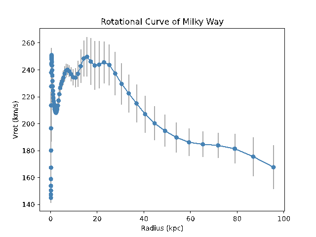
Figure 5. Scatter plot of rotation curves in the Milky Way using values from [5].

With our velocity functions for the bulge, disk, and DM halo, we seek to use equation 5 to find the ultimate rotation velocity of the galaxy. To do this, we manually alter the function parameters to fit the total Galactical velocity graph. In the end, we estimate a best fit scale radius of 10.0 kpc for the DM halo, normalization constant \( 2.6×{10^{40}} \) GeV/ \( {cm^{3}} \) and scale radius 0.13 kpc for the bulge, and normalization constant \( 0.75×{10^{3}} \) and scale radius 3.0 kpc for the disk. The compiled graph is shown below in figure 6.

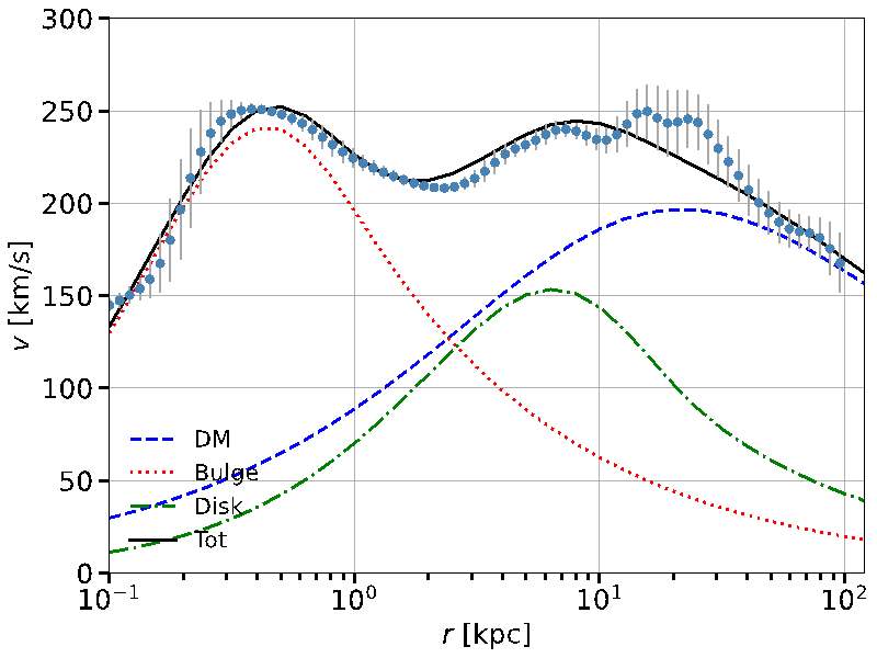
Figure 6. Best fit \( {V_{rot}} \) line using manually altered parameters.

1.6 Best fit parameters/error

We follow a similar procedure for the final part of this study, except this time using the python package Minuit to calculate the precise \( {ρ_{⨀}} \) as well as normalization and scale radius values for the best fit rotation velocity function. As mentioned earlier, we first increment the \( {ρ_{⨀}} \) value by 0.1 from 0.3 GeV/ \( {cm^{3}} \) to 0.6 GeV/ \( {cm^{3}} \) , not including it as a parameter. The obtained Minuit results for each value are presented in table 3. The compiled best fit graphs for each are also displayed in figure 7. As shown, the smallest value of \( {χ^{2}} \) occurred when \( {ρ_{⨀}} \) was equal to 0.5 GeV/ \( {cm^{3}} \) .

Table 3. Resulting best fit scale radii parameters and \( {χ^{2}} \) when \( {ρ_{⨀}} \) = 0.3, 0.4, 0.5, and 0.6 GeV/ \( {cm^{3}} \) .

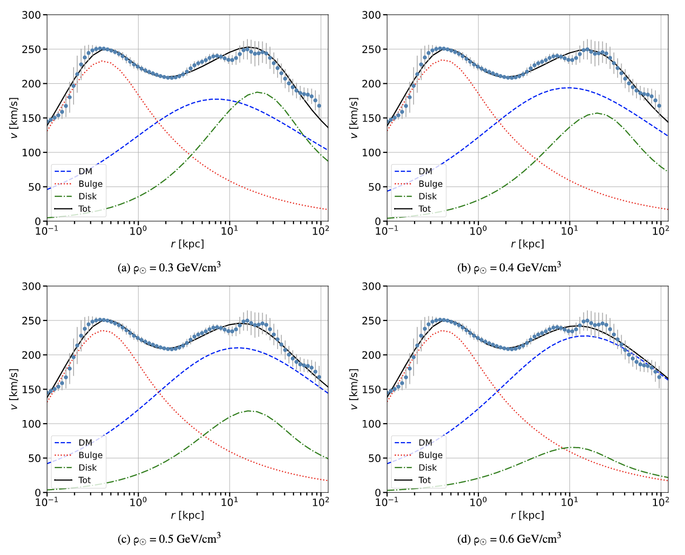
Figure 7. Compiled best fit of the rotational velocity \( {V_{rot}} \) with different values of \( {ρ_{⨀}} \) : 0.3, 0.4, 0.5, and 0.6 GeV/ \( {cm^{3}} \) .

Our final step is to use the computer program to gauge the precise best fit \( {ρ_{⨀}} \) by including it as a parameter. The resulting values are listed in table 4, with three columns for the NFW, Einasto, and Burkert profiles. NFW had the smallest \( {χ^{2}} \) of 38.72 with \( {ρ_{⨀}} \) = 0.53 GeV/ \( {cm^{3}} \) and a scale radius \( {r_{DM}} \) = 6.11 kpc. For the Einasto profile, \( {ρ_{⨀}} \) was 0.47 and the scale radius 15.79 kpc with an overall \( {χ^{2}} \) of 53.54, while Burkert returned a \( {ρ_{⨀}} \) of 0.69 and scale radius of 4.37 kpc at a \( {χ^{2}} \) of 40.03. The best fit graphs for each of the DM profiles are presented side by side in figure 8.

Table 4. Resulting scale radii, \( {ρ_{⨀}} \) , and \( {χ^{2}} \) values for NFW, Einasto, and Burkert profiles when including \( {ρ_{⨀}} \) as a parameter.

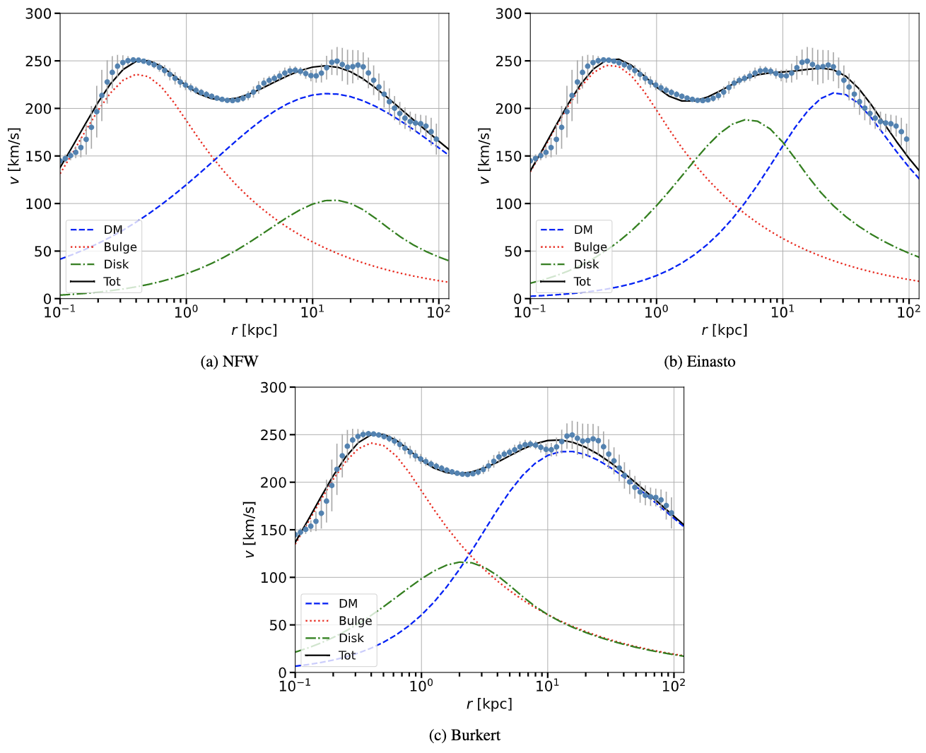
Figure 8. Compiled best fit \( {V_{rot}} \) graphs with \( {ρ_{⨀}} \) as a parameter for NFW, Einasto, and Burkert profiles.

6. Conclusions

In this paper, we employed two different techniques to determine the DM density distribution in the Milky Way. First, we mathematically rewrote DM profiles to obtain values for the parameters \( {r_{s}} \) and \( {ρ_{s}} \) , then calculated the best fit \( {ρ_{s}} \) – based on the Galactic rotation velocity data – both manually and systematically, the latter with the Python minimization package Minuit. For all procedures, we demonstrated the need of DM to explain the gravitational dynamic in the Galaxy. In particular, we determined a typical scale radius of 5-20 kpc and a local DM density of the order of 0.5-0.7 GeV/ \( {cm^{3}} \) .

References

[1]. Bertone G and Hooper D 2018 Rev. Mod. Phys. 90 045002.
[2]. Van Albada T S, Bahcall J N, Begeman K and Sancisi R 1985 Astrophys. J. 295 305.
[3]. Cirelli M, Gorcella G, Hektor A, Hutsi G, Kadastik M, Panci P, Raidal M, Sala F and Strumia A 2011 JCAP 03 051.
[4]. De Salas P, Malhan K, Freese K, Hattori K and Valluri M 2019 Journal of Cosmology and Astroparticle Physics 2019 037.
[5]. Sofue Y 2020 Galaxies 8 37.
[6]. Sofue Y 2016 Publications of the Astronomical Society of Japan 69 R1.
Cite this article
Lu,Y. (2023). Density of dark matter in the Milky Way. Theoretical and Natural Science,11,36-46.
Data availability
The datasets used and/or analyzed during the current study will be available from the authors upon reasonable request.
Disclaimer/Publisher's Note
The statements, opinions and data contained in all publications are solely those of the individual author(s) and contributor(s) and not of EWA Publishing and/or the editor(s). EWA Publishing and/or the editor(s) disclaim responsibility for any injury to people or property resulting from any ideas, methods, instructions or products referred to in the content.
About volume
Volume title: Proceedings of the 2023 International Conference on Mathematical Physics and Computational Simulation
© 2024 by the author(s). Licensee EWA Publishing, Oxford, UK. This article is an open access article distributed under the terms and
conditions of the Creative Commons Attribution (CC BY) license. Authors who
publish this series agree to the following terms:
1. Authors retain copyright and grant the series right of first publication with the work simultaneously licensed under a Creative Commons
Attribution License that allows others to share the work with an acknowledgment of the work's authorship and initial publication in this
series.
2. Authors are able to enter into separate, additional contractual arrangements for the non-exclusive distribution of the series's published
version of the work (e.g., post it to an institutional repository or publish it in a book), with an acknowledgment of its initial
publication in this series.
3. Authors are permitted and encouraged to post their work online (e.g., in institutional repositories or on their website) prior to and
during the submission process, as it can lead to productive exchanges, as well as earlier and greater citation of published work (See
Open access policy for details).