1. Introduction

The waterjet propulsion system is a marine propulsion device that generates reaction thrust by ejecting a jet of water. It consists of an inlet duct, an impeller, a stator with guide vanes, a nozzle, steering devices, and a reversing bucket. It is an internal flow device, transmitting thrust not only through the shaft but also through the boundary and internal structures [1]. The applications of waterjet propulsion systems on modern high-speed vessels have been growing rapidly since the 1980s, due to their high efficiency, reduced drafts, and improved maneuverability [1-2].

Efficiency is a key aspect of the performance of a waterjet propulsion unit, which is affected by multiple factors including the structures of the inlet duct, the nozzle, the relative motion between the ship and water, as well as the cavitation in the unit. Using numerical and experimental methods, particularly computational fluid dynamics (CFD), a number of studies have been conducted investigating the influences of various factors on the efficiency and flow characteristics of waterjet propulsion systems. Ding et al. [3] determined the flow loss in a flush-type inlet duct of a waterjet propulsion unit to be 0.05-0.12 by numerical simulation, in which a scalar quantity was introduced to mark the stream tube. Jiao et al. [4] carried out a comprehensive optimization of the geometry of the inlet passage of a waterjet propulsion system using the CFD method. Xu et al. [5] conducted a numerical analysis of the effects of ship motions relative to water and impeller shaft rotation on the hydrodynamic performance of the inlet duct of a waterjet propulsion unit. Xia et al. [6] numerically analyzed the flow separation and rotating stall occurring near the impeller and guide vanes in a waterjet propulsion system. Huang et al. [7] carried out theoretical, numerical, and experimental investigations of a submerged conical nozzle to determine the relationships between reaction thrust and various operating conditions and the nozzle geometry for minimum energy loss. Yang et al. [8] conducted an optimization of the nozzle of a waterjet propulsion unit with a positive displacement pump using CFD simulation. Wang et al. [9] optimized the outlet area, shape, and transition curve of the nozzle of a waterjet propulsion unit under a fixed flow rate condition by CFD analysis. Jiao et al. [10] numerically simulated the cavitation process in a waterjet propulsion pump and the whole system. All the above-mentioned numerical studies included experimental validations.

Table 1. Nomenclature symbols.

The nozzle of a waterjet propulsion system plays a crucial role in generating thrust. It accelerates the flow and converts the static pressure of water flow into dynamic pressure, which considerably raises the kinetic energy and momentum of the water to create reactive thrust. Using the computational fluid dynamics method, this study investigates the influences of the nozzle shape and outlet area on the nozzle efficiency and overall efficiency of a waterjet propulsion unit. The performances of cylindrical and conical nozzles with 5 different outlet areas are simulated and compared in order to determine the optimal outlet area and nozzle shape.

2. Simulation setup

2.1. Computational domain

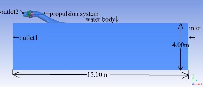
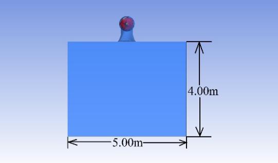
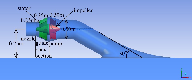
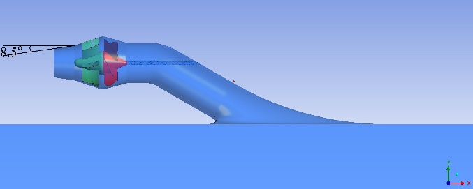
The computational fluid dynamics simulation was conducted using the fluid simulation software Ansys Fluent. As shown in Fig. 1 and Fig. 2, the computational domain includes the propulsion unit and the external water body below the vessel. There are 1 inlet and 2 outlets in the entire domain: the inlet of the water body, the outlet of the water body “outlet1”, and the nozzle outlet of the propulsion unit “outlet2”. The inlet duct diameter is set as 0.50m and the nozzle outlet diameter is varied across different simulation cases. The water body was 15.00m in length, 5.00m in width, and 4.00m in height. The dimensions of the propulsion units with cylindrical and conical nozzles are depicted in Fig. 3 and Fig. 4 respectively. The dip angle of the inlet duct is \( 30° \) and the half angles of all the conical nozzles are \( 8.5° \) . The lengths of the propulsion pump, the guide vane section, and the nozzle are 0.30m, 0.35m, and 0.25m respectively.

There are 2 cell zones in the mesh generated: a rotating cell zone surrounding the rotating impeller and a stationary cell zone consisting of the rest of the flow field outside the rotating zone. The two cell zones are divided by an interface on which the mesh in the two zones can slide freely relative to each other. The impeller has a fixed rotating speed of 1800rpm (188.5rad/s), which is also the rotating speed of the rotating cell zone. Poly-hex-core cells are generated in the mesh, with cell sizes of 0.30m in the water body, 0.02m in the stationary region in the propulsion unit, and 0.005m in the rotating cell zone. The total number of cells varies between \( 1.8×{10^{6}} \) and \( 2.1×{10^{6}} \) over different cases.

2.2. Governing equations and numerical models

Reynolds averaging is adopted to account for the turbulent flow, which breaks the velocity \( u \) into a time-averaged mean component \( \bar{u} \) and a fluctuating component \( u \prime \) :

\( {u_{i}}={\bar{u}_{i}}+u_{i}^{ \prime } \) (1)

The continuity equation used in the simulation is written in the Cartesian tensor form as:

\( \frac{∂ρ}{∂t}+\frac{∂(ρ{\bar{u}_{i}})}{∂{x_{i}}}=0 \) (2)

The momentum governing equation is the Reynolds-averaged Navier-Stokes equation, which is written as follows in the Cartesian tensor form:

\( \frac{∂(ρ{\bar{u}_{i}})}{∂t}+\frac{∂(ρ{\bar{u}_{i}}{\bar{u}_{j}})}{∂{x_{j}}}=-\frac{∂p}{∂{x_{i}}}+\frac{∂}{∂{x_{j}}}[μ(\frac{∂{\bar{u}_{i}}}{∂{x_{j}}}+\frac{∂{\bar{u}_{j}}}{∂{x_{i}}}-\frac{2}{3}{δ_{ij}}\frac{∂{\bar{u}_{k}}}{∂{x_{k}}})]+\frac{∂}{∂{x_{j}}}(-ρ\bar{u_{i}^{ \prime }u_{j}^{ \prime }}) \) (3)

The SST k- \( ω \) turbulence model [11] is adopted in the simulation, the transport equations of which are written as follows in the Cartesian tensor form:

\( \frac{∂(ρk)}{∂t}+\frac{∂(ρk{\bar{u}_{i}})}{∂{x_{i}}}=\frac{∂}{∂{x_{j}}}({Γ_{k}}\frac{∂k}{∂{x_{j}}})+{G_{k}}-{Y_{k}}+{S_{k}} \) (4)

\( \frac{∂(ρω)}{∂t}+\frac{∂(ρω{\bar{u}_{i}})}{∂{x_{i}}}=\frac{∂}{∂{x_{j}}}({Γ_{ω}}\frac{∂ω}{∂{x_{j}}})+{G_{ω}}-{Y_{ω}}+{D_{ω}}+{S_{ω}} \) (5)

Where \( {Γ_{k}} \) , \( {Γ_{ω}} \) , \( {G_{k}} \) , \( {G_{ω}} \) , \( {Y_{k}} \) , \( {Y_{ω}} \) , \( {S_{k}} \) , and \( {S_{ω}} \) represent the effective diffusivity, generation, dissipation, and user-defined source terms of the turbulent kinetic energy and the specific dissipation rate respectively, and \( {D_{ω}} \) denotes the cross-diffusion term.

The Schnerr-Sauer cavitation model [12] is utilized to account for the cavitation occurring in the propulsion unit. The governing equations are given as follows:

\( \frac{∂(α{ρ_{v}})}{∂t}+∇∙(α{ρ_{v}}\vec{V})=R \) (6)

\( {R_{B}}={(\frac{3α}{4π(1-α){n_{b}}})^{\frac{1}{3}}} \) (7)

\( R=\lbrace \begin{array}{c} {F_{vap}}\frac{{ρ_{v}}{ρ_{l}}}{ρ}α(1-α)\frac{3}{{R_{B}}}\sqrt[]{\frac{2}{3}\frac{({p_{v}}-p)}{{ρ_{l}}}}, p≤{p_{v}} \\ -{F_{cond}}\frac{{ρ_{v}}{ρ_{l}}}{ρ}α(1-α)\frac{3}{{R_{B}}}\sqrt[]{\frac{2}{3}\frac{({p-p_{v}})}{{ρ_{l}}}}, p \gt {p_{v}} \end{array} \rbrace \) (8)

Where \( α \) is the vapor volume fraction, \( ρ \) is the density of the liquid-vapor mixture, \( {ρ_{v}} \) is the vapor phase density, \( {ρ_{l}} \) is the liquid phase density, \( R \) is the mass transfer rate from the liquid phase to the vapor phase, \( {R_{B}} \) is the vapor bubble radius, \( {n_{b}} \) is the bubble number per unit liquid volume, \( p \) is the mixture pressure, \( {p_{v}} \) is the vapor pressure, and \( {F_{vap}} \) and \( {F_{cond}} \) are the empirical calibration coefficients of evaporation and condensation respectively.

2.3. Boundary conditions

The non-slip condition is applied to all solid walls of the propulsion unit and the top boundary of the water body to simulate the boundary layer formed on the solid walls of the propulsion unit and the bottom of the hull. The condition of zero shear stress is imposed on the sides and bottom of the water body. The inlet is set as a velocity inlet with a uniform inflow velocity of 20.58m/s, which is the assumed sailing speed of the ship. The nozzle outlet is assumed to be exposed rather than submerged since the nozzles of actual waterjet propulsion systems are above the waterline when operating at high sailing speeds due to the hollow of water immediately behind the stern of a vessel sailing at high speeds, and the effect of gravity is neglected in the simulation due to its relatively minor effect on the flow field. The two outlets, “outlet1” and “outlet2”, are both pressure outlets with a gauge static pressure of 0Pa, since the ambient pressures in both the air and water are equal to the atmospheric pressure when gravity is neglected.

3. Results and discussions

3.1. Simulation cases

As shown in Table 2, the waterjet propulsion units with 10 different geometries are analyzed through CFD simulation. In cases 1-5, the propulsion systems are equipped with cylindrical nozzles and the nozzle outlet areas \( {A_{out}} \) are 60%, 50%, 40%, 30%, and 25% of the inlet duct area \( {A_{in}} \) respectively. In cases 6-10, the propulsion systems are equipped with conical nozzles with the same set of outlet areas.

Table 2. Summary of simulated cases.

3.2. Influences of nozzle shape and outlet area on nozzle efficiency

The nozzle efficiency is calculated using the following formula:

\( {η_{n}}=\frac{{\dot{E}_{out}}}{{\dot{E}_{in}}}=\frac{\dot{m}g{H_{out}}}{\dot{m}g{H_{in}}}=\frac{{H_{out}}}{{H_{in}}}×100\% \) (9)

Where \( {η_{n}} \) is the nozzle efficiency, \( {H_{in}} \) is the mass-weighted average total head at the nozzle inlet, and \( {H_{out}} \) is the total head at the nozzle outlet.

The mass-weighted average value of a scalar quantity at a surface in the flow field is calculated as follows:

\( \bar{ϕ}=\frac{\int ρϕ|\vec{V}∙d\vec{A}|}{\int ρ|\vec{V}∙d\vec{A}|}=\frac{\sum _{i=1}^{n}{ρ_{i}}{ϕ_{i}}|\vec{{V_{i}}}∙\vec{{A_{i}}}|}{\sum _{i=1}^{n}{ρ_{i}}|\vec{{V_{i}}}∙\vec{{A_{i}}}|} \) (10)

Where \( ϕ \) is a general scalar variable, \( d\vec{A} \) is the normal vector of a differential area of the surface with a magnitude of the differential area.

Table 3 and Fig. 5 illustrate the variations of nozzle efficiency with the outlet areas of both cylindrical and conical nozzles. The nozzle efficiency of a cylindrical nozzle increases consistently with the nozzle outlet area, from 82.96% at the outlet area of \( 25\%{A_{in}} \) to 93.17% at the outlet area of \( 60\%{A_{in}} \) . The growth of the nozzle efficiency of a cylindrical nozzle is significant as the outlet area increases from \( 25\%{A_{in}} \) to \( 40\%{A_{in}} \) and relatively moderate as the outlet area rises from 40% to 60% of the inlet duct area. The nozzle efficiency of a conical nozzle shows a general slightly increasing trend involving considerable fluctuations with the outlet area, with the minimum nozzle efficiency of 92.23% occurring at the outlet area of \( 30\%{A_{in}} \) and the maximum of 96.02% occurring at the outlet area of \( 60\%{A_{in}} \) . The efficiencies of the conical nozzles are higher than those of the cylindrical nozzles across the whole range of nozzle outlet areas investigated.

Fig. 6 and Fig. 7 depict the change in the mass-weighted average total head at a cross-sectional plane of a nozzle with the longitudinal distance of the plane from the nozzle inlet plane. The total heads at the inlet, outlet, and three quartiles of a nozzle are calculated. \( {H_{in}} \) represents the total head at the nozzle inlet plane and \( {H_{x}} \) represents the total head at a cross-section of the nozzle at \( x \) meters from the nozzle inlet plane. The total head decreases steeply in the first quarter of both the cylindrical and conical nozzles and the drop in the total head tends to be more drastic in the nozzles with smaller outlet areas and in the cylindrical nozzles. An approximately linear descent of the total head takes place throughout the second and third quarters of both the cylindrical and conical nozzles. In these two quarters, the total head declines more significantly in the nozzles with smaller outlet areas and decreases more in conical nozzles than in cylindrical ones at the outlet areas of \( 60\%{A_{in}} \) and \( 50\%{A_{in}} \) . In the last quarter of the cylindrical nozzles, the total head declines slightly in the nozzles with outlet areas of \( 60\%{A_{in}} \) and \( 50\%{A_{in}} \) and plunges considerably in the nozzles with outlet areas of no more than 40% of the inlet duct area. In the last quarter of the conical nozzles, the total head increases slightly except for the one with an outlet area of 25% of the inlet duct area.

Table 3. Nozzle efficiency in each case.

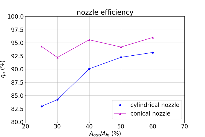
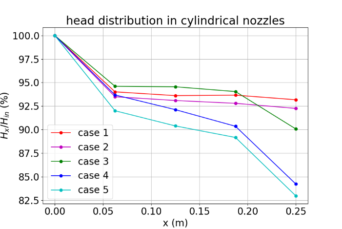
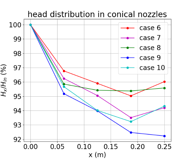
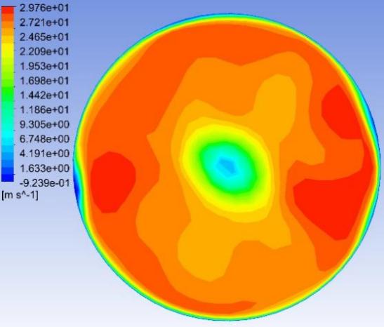
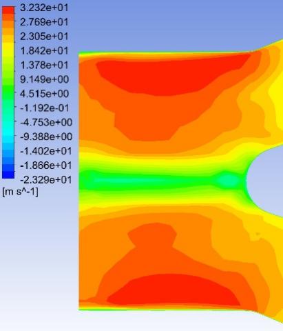
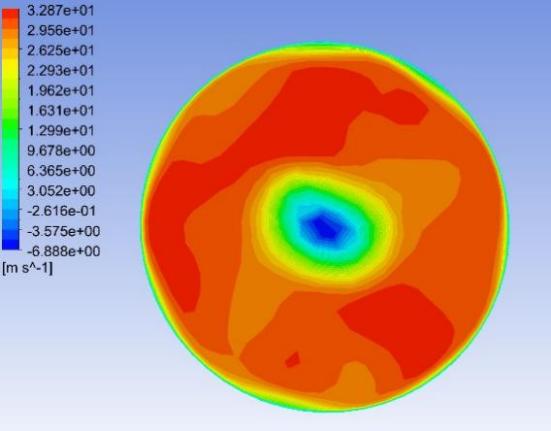
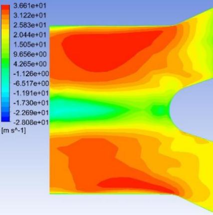
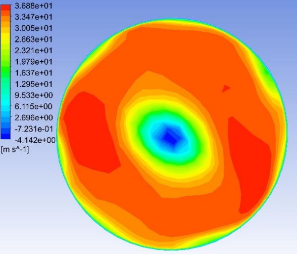
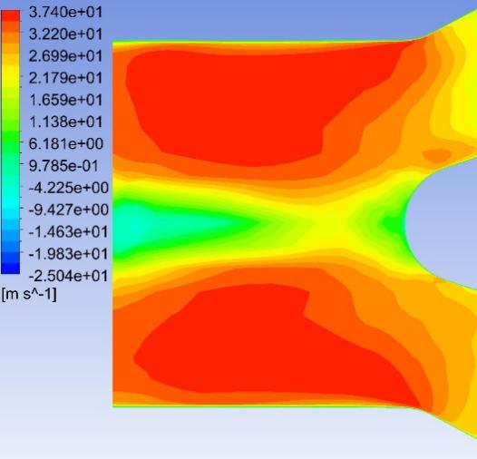
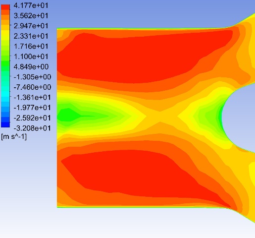
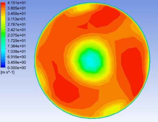
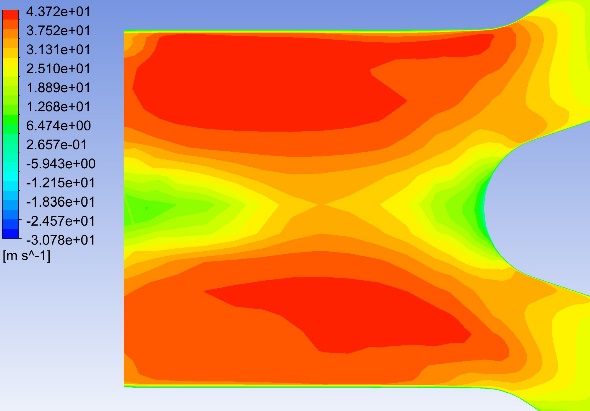
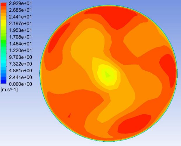
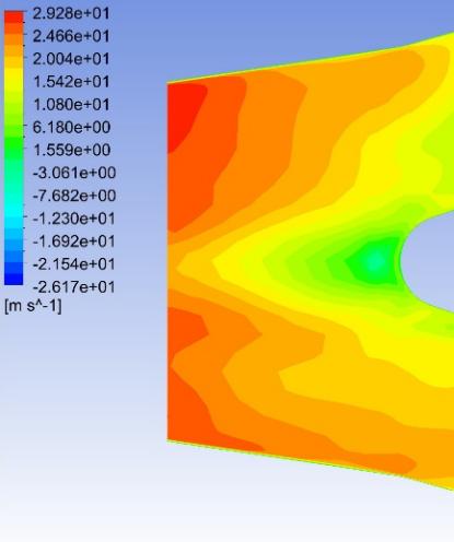
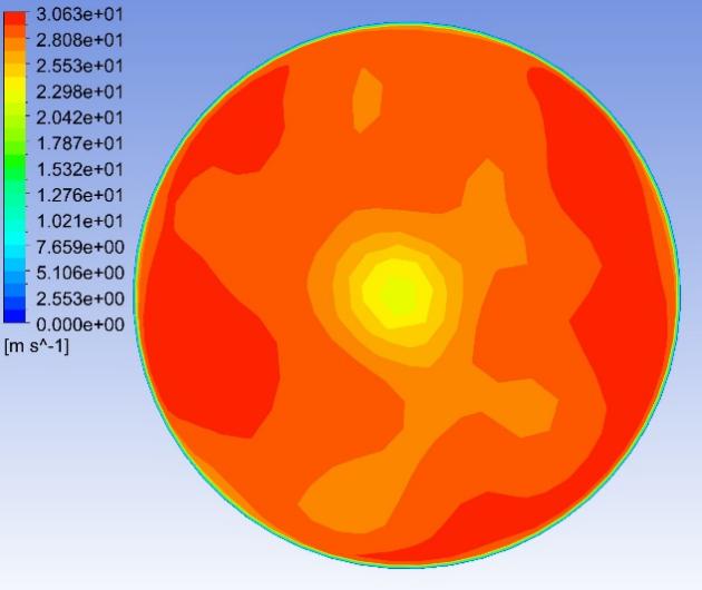
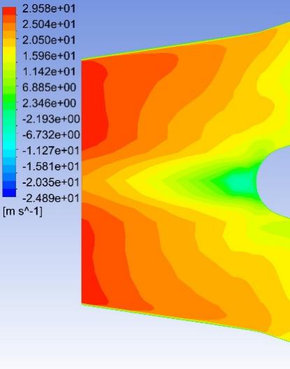
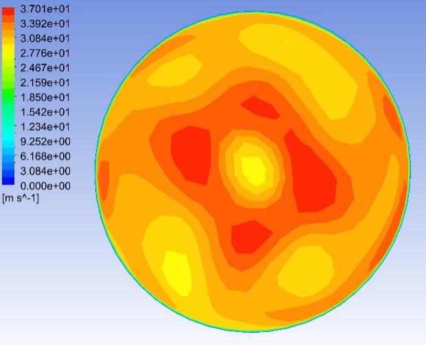
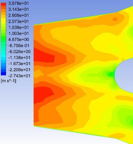
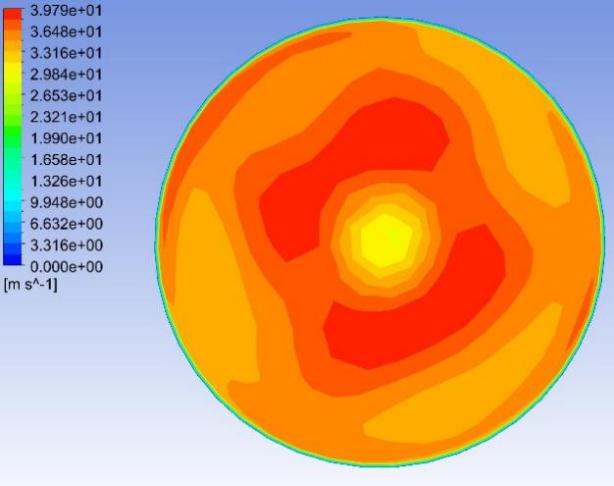
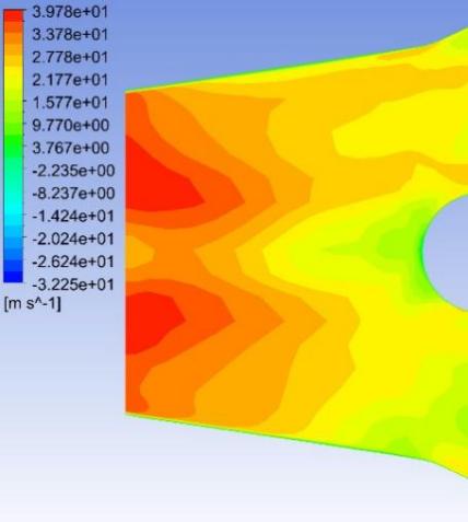
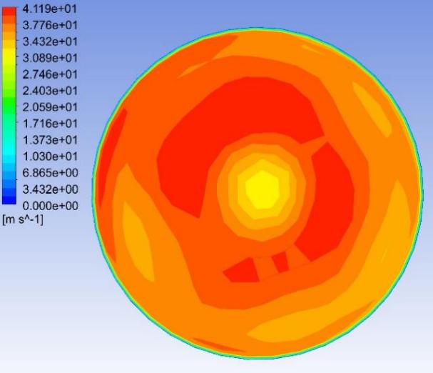
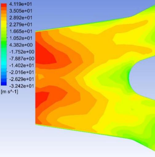
Fig. 8–Fig. 27 display the axial velocity contours of the cylindrical and conical nozzles at the outlet plane and the longitudinal section of the nozzles. In a cylindrical nozzle, there is a low-velocity region at the center of the nozzle, coincident with the wake behind the stator hub, surrounded by an annular high-velocity region around the nozzle periphery. At outlet areas of \( 60\%{A_{in}} \) and \( 50\%{A_{in}} \) , the central low-velocity region and the annular high-velocity region do not mix with each other. At outlet areas smaller than or equal to \( 40\%{A_{in}} \) , the annular high-velocity region briefly mixes with the wake behind the stator hub before the central low-velocity region expands again. In the conical nozzles with outlet areas of \( 60\%{A_{in}} \) and \( 50\%{A_{in}} \) , a large annular high-velocity region surrounds a central low-velocity region. At outlet areas of 25%-40% of the inlet duct area, 3 regions with distinctly different velocities can be observed in a conical nozzle: the central region with low axial velocity, the inner annular region with the maximum velocity, and the outer annular region with intermediate axial velocity. The annular high-velocity region apparently mixes with the wake behind the stator hub in a conical nozzle, thanks to the contractionary effect of the nozzle on the flow direction, which makes the central low-velocity regions in conical nozzles smaller and less distinct than those in cylindrical nozzles.

Some possible reasons for the variations of the nozzle efficiency with the nozzle shapes and nozzle outlet areas are suggested by the above-mentioned observations. There is an abrupt change in the flow direction at the transition between the guide vane section and the nozzle, which incurs energy loss due to turbulence and viscosity. The energy loss is greater in nozzles with smaller outlet areas and in cylindrical nozzles than that in conical nozzles, since the changes in flow direction are more drastic in these cases. This accounts for the more drastic decline of the total head in the first quarter of the nozzles with smaller outlet areas and in cylindrical nozzles. The approximately linear descent of the total head in the second and third quarters of the nozzles suggests that the major source of energy loss in this section of the nozzles is the skin friction on the nozzle walls. The skin friction is more influential to the flow field in nozzles with smaller outlet areas, which leads to a steeper decline in the total head in the nozzles with smaller outlet areas. In the last quarter of the cylindrical nozzles with outlet areas smaller than or equal to 40% of the inlet duct area, the drastic drop of the total head is possibly associated with the expansion of the low-axial-velocity region at the center of the nozzles. The slight rise of the total head in the last quarter of the conical nozzles with outlet areas greater than 30% of the inlet duct area is potentially associated with the mixing between the annular high-velocity region and the central low-velocity region near the nozzle outlet.

3.3. Influences of nozzle shape and outlet area on overall efficiency

The thrust of the waterjet propulsion system is obtained by considering the propulsion unit and the ingested stream tube as a control volume and calculating the difference between the inflow momentum flux and the exit momentum flux. The thrust is given by the following formula:

\( T=\dot{m}{V_{out}}-\dot{m}{V_{in}}=ρ\dot{Q}[{V_{out}}-(1-w){V_{s}}] \) (11)

\( {V_{in}}=(1-w){V_{s}} \) (12)

Where \( w \) is the wake fraction assumed to be 5%.

Thus, the overall efficiency can be calculated as follows:

\( {η_{o}}=\frac{{P_{out}}}{{P_{s}}}=\frac{T{V_{s}}}{τΩ}=\frac{ρ\dot{Q}{V_{s}}[{V_{out}}-(1-w){V_{s}}]}{τΩ} \) (13)

Table 4 and Fig. 28 illustrate the variations in the overall efficiency of a waterjet propulsion system with the nozzle shape and the outlet area. The overall efficiency of a waterjet propulsion system with a cylindrical nozzle increases consistently with the nozzle outlet area from 31.22% to 54.43% as the outlet area increases from \( 25\%{A_{in}} \) to \( 50\%{A_{in}} \) . Then it decreases to 50.82% as the nozzle outlet area rises to \( 60\%{A_{in}} \) . The overall efficiency of a waterjet propulsion unit with a conical nozzle decreases from 37.15% to 33.10% as the nozzle outlet area increases from \( 25\%{A_{in}} \) to \( 30\%{A_{in}} \) and then soars to 51.15% at the outlet area of \( 40\%{A_{in}} \) , followed by a gentle linear growth to 54.42% as the outlet area reaches 60% of the inlet duct area. The overall efficiency of the waterjet propulsion unit equipped with the cylindrical nozzle with an outlet area of \( 50\%{A_{in}} \) and that of the propulsion unit equipped with the conical nozzle with an outlet area of \( 60\%{A_{in}} \) are almost equal and both of them can be considered the maximum overall efficiency. The overall efficiencies of the propulsion units with conical nozzles are generally higher than those of the propulsion units with cylindrical nozzles.

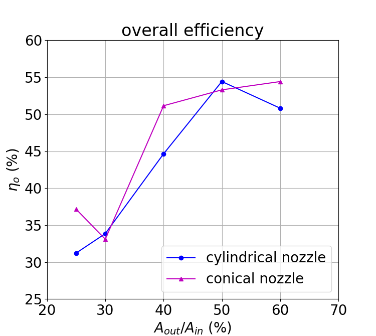
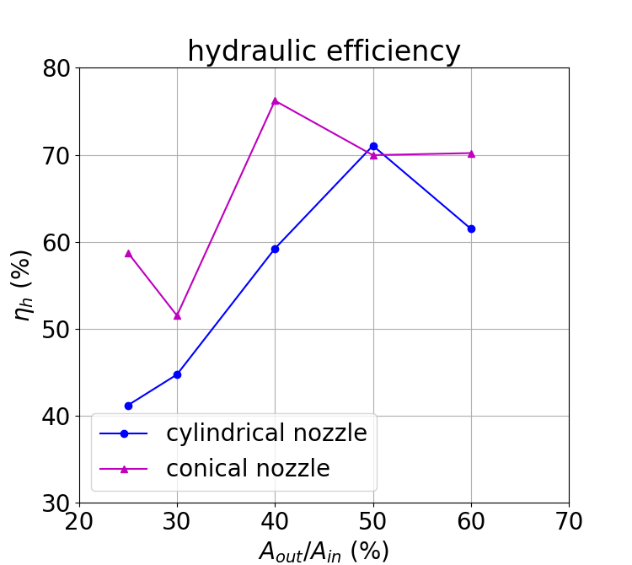
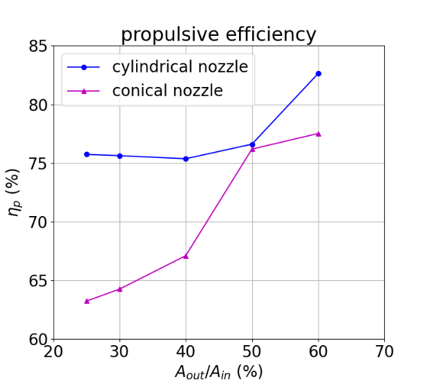
Table 4. Overall efficiency in each case.

Table 5. Hydraulic efficiency in each case.

Table 6. Propulsive efficiency in each case.

The hydraulic efficiency and propulsive efficiency of the waterjet propulsion systems are also investigated. The hydraulic efficiency denotes the proportion of shaft work of the impeller being converted to the mechanical energy of the water, which is calculated as follows:

\( {η_{h}}=\frac{\dot{m}gΔH}{{P_{s}}}=\frac{\dot{m}gΔH}{τΩ} \) (14)

The propulsive efficiency represents the proportion of the hydraulic power being converted to the propulsive power of the ship, which is calculated as follows:

\( {η_{p}}=\frac{T{V_{s}}}{\dot{m}gΔH}=\frac{\dot{m}({V_{out}}-(1-w){V_{s}}){V_{s}}}{\dot{m}gΔH}=\frac{({V_{out}}-(1-w){V_{s}}){V_{s}}}{gΔH} \) (15)

The following relationship exists between overall efficiency, hydraulic efficiency, and propulsive efficiency:

\( {η_{o}}={η_{h}}{η_{p}} \) (16)

Table 5, Fig. 29, and Table 6, Fig. 30 illustrate the hydraulic and propulsive efficiencies respectively of waterjet propulsion systems with different nozzle shapes and outlet areas. The waterjet propulsion systems with conical nozzles are generally more desirable in terms of hydraulic efficiency and the waterjet propulsion systems with cylindrical nozzles are consistently more desirable in terms of propulsive efficiency. The trend of the overall efficiency of a waterjet propulsion system equipped with a cylindrical nozzle with its outlet area closely resembles the trend of its hydraulic efficiency with its outlet area. At outlet areas \( 25\%{A_{in}} \) – \( 40\%{A_{in}} \) , the overall efficiency of a propulsion unit with a conical nozzle varies with outlet areas in a similar way as the variation of the hydraulic efficiency. At outlet areas of \( 50\%{A_{in}} \) and \( 60\%{A_{in}} \) , the overall efficiency of a propulsion unit with a conical nozzle is more affected by the propulsive efficiency, since the overall efficiency continues to increase despite the descent of the hydraulic efficiency. Therefore, the major source of energy loss in a waterjet propulsion system is the internal loss of the mechanical energy of water, while the reduced kinetic energy carried by the exit flow considerably improves the overall efficiencies of the propulsion units equipped with conical nozzles with relatively large outlet areas.

4. Conclusion

In order to study the influences of the nozzle shape and outlet area of a waterjet propulsion system on its efficiency, the flow fields in the waterjet propulsion systems equipped with cylindrical and conical nozzles with 5 different outlet areas are numerically simulated using the method of computational fluid dynamics. The variations of the nozzle efficiency and the overall efficiency with the nozzle shape and outlet area are thoroughly investigated. The maximum nozzle efficiency is 96.02% occurring in the conical nozzle with an outlet area of 60% of the inlet duct area. The nozzle efficiencies of conical nozzles are consistently higher than those of cylindrical nozzles across the whole range of nozzle outlet areas investigated in this study, and the nozzle efficiency has a general increasing trend with the nozzle outlet area. The viscous and turbulent energy loss incurred by the abrupt change in the flow direction at the transition between the guide vane section and the nozzle and the skin friction on nozzle walls are major contributing factors to the energy loss in a nozzle. The overall efficiency of the waterjet propulsion system equipped with the cylindrical nozzle with an outlet area of 50% of the inlet duct area and that of the propulsion system equipped with the conical nozzle with an outlet area of 60% of the inlet duct area are the maximum and almost equal to each other, being 54.43% and 54.42% respectively. The overall efficiency of a propulsion unit equipped with a conical nozzle generally increases with the nozzle outlet area, whereas the overall efficiency of a propulsion unit equipped with a cylindrical nozzle increases with outlet area at smaller outlet areas and decreases when the outlet area exceeds 50% of the inlet duct area. The conical nozzles are generally more desirable than cylindrical nozzles in terms of overall efficiency. The hydraulic efficiency is the dominating factor affecting the overall efficiency, while the propulsive efficiency also exerts influence on the overall efficiency to some extent when the propulsion unit is equipped with a conical nozzle with a relatively large outlet area.

This study is subject to certain limitations. Firstly, the simulated results are not confirmed by experimental validation, which means the simulated flow characteristics might involve some inaccuracies. In addition, the wake fraction is set as the empirical value of 5% rather than calculated from the flow field. Despite these limitations, the CFD simulation sheds light on the influences of the nozzle shape and the outlet area of a waterjet propulsion system on the nozzle efficiency and overall efficiency and explores the possible underlying reasons behind the influences, which could offer some insights into the design of future marine waterjet propulsion systems.

References

[1]. Bulten, N. W. H. (2006). Numerical analysis of a waterjet propulsion system. Dissertation Abstracts International, 68(02).
[2]. Carlton, J. S. (2019). Waterjet propulsion. Marine Propellers and Propulsion, 399–408. https://doi.org/10.1016/b978-0-08-100366-4.00016-x.
[3]. Ding, J. M. and Wang, Y. S. (2010). Research on flow loss of inlet duct of marine waterjets. Journal of Shanghai Jiaotong University (Science), 15(2), 158–162. https://doi.org/10.1007/s12204-010-8130-x.
[4]. Jiao, W., Cheng, L., Zhang, D., Zhang, B., Su, Y. and Wang, C. (2019). Optimal design of inlet passage for waterjet propulsion system based on flow and geometric parameters. Advances in Materials Science and Engineering, 2019, 1–21. https://doi.org/10.1155/2019/2320981.
[5]. Xu, H. and Zou, Z. (2021). Numerical simulation of the flow in a waterjet intake under different motion conditions. Journal of Shanghai Jiaotong University (Science), 27(3), 356–364. https://doi.org/10.1007/s12204-021-2321-5.
[6]. Xia, C., Cheng, L., Luo, C., Jiao, W. and Zhang, D. (2019). Hydraulic characteristics and measurement of rotating stall suppression in a waterjet propulsion system. Transactions of FAMENA, 42(4), 85–100. https://doi.org/10.21278/tof.42408.
[7]. Huang, G. Q., Yang, Y. S., Li, X. H. and Zhu, Y. Q. (2009). Reaction thrust of water jet for conical nozzles. Journal of Shanghai University (English Edition), 13(4), 305–310. https://doi.org/10.1007/s11741-009-0411-1.
[8]. Yang, Y. S., Xie, Y. C. and Nie, S. L. (2014). Nozzle optimization for water jet propulsion with a positive displacement pump. China Ocean Engineering, 28(3), 409–419. https://doi.org/10.1007/s13344-014-0033-4.
[9]. Wang, C., He, X., Cheng, L., Luo, C., Xu, J., Chen, K. and Jiao, W. (2019). Numerical simulation on hydraulic characteristics of nozzle in Waterjet Propulsion System. Processes, 7(12), 915–935. https://doi.org/10.3390/pr7120915.
[10]. Jiao, W., Cheng, L., Xu, J. and Wang, C. (2019). Numerical Analysis of two-phase flow in the cavitation process of a waterjet propulsion pump system. Processes, 7(10), 690–712. https://doi.org/10.3390/pr7100690.
[11]. Menter, F. R. (1994). Two-equation eddy-viscosity turbulence models for engineering applications. AIAA Journal, 32(8), 1598–1605. https://doi.org/10.2514/3.12149.
[12]. Schnerr, G. H. and Sauer, J. (2001). Physical and numerical modeling of unsteady cavitation dynamics. In Fourth international conference on multiphase flow (Vol. 1). New Orleans, LO, USA: ICMF New Orleans.
Cite this article
Wei,M. (2023). Numerical analysis of the effects of the nozzle shape and outlet area of a waterjet propulsion system on its efficiency. Theoretical and Natural Science,11,47-59.
Data availability
The datasets used and/or analyzed during the current study will be available from the authors upon reasonable request.
Disclaimer/Publisher's Note
The statements, opinions and data contained in all publications are solely those of the individual author(s) and contributor(s) and not of EWA Publishing and/or the editor(s). EWA Publishing and/or the editor(s) disclaim responsibility for any injury to people or property resulting from any ideas, methods, instructions or products referred to in the content.
About volume
Volume title: Proceedings of the 2023 International Conference on Mathematical Physics and Computational Simulation
© 2024 by the author(s). Licensee EWA Publishing, Oxford, UK. This article is an open access article distributed under the terms and
conditions of the Creative Commons Attribution (CC BY) license. Authors who
publish this series agree to the following terms:
1. Authors retain copyright and grant the series right of first publication with the work simultaneously licensed under a Creative Commons
Attribution License that allows others to share the work with an acknowledgment of the work's authorship and initial publication in this
series.
2. Authors are able to enter into separate, additional contractual arrangements for the non-exclusive distribution of the series's published
version of the work (e.g., post it to an institutional repository or publish it in a book), with an acknowledgment of its initial
publication in this series.
3. Authors are permitted and encouraged to post their work online (e.g., in institutional repositories or on their website) prior to and
during the submission process, as it can lead to productive exchanges, as well as earlier and greater citation of published work (See
Open access policy for details).