1. Introduction

Computers are commonly used production tools. From 1946 to the present, traditional computers have gone through four stages of development, namely vacuum tube computer, Transistor computer, Small and medium-scale integrated circuit computer, and Large-scale and very large-scale integrated circuit computers [1]. Today's traditional computers can meet the daily needs of most people, but there are limitations. The first is computing speed. While traditional computers are fast, they are still limited when processing large amounts of data. The second is storage capacity. The storage capacity of traditional computers is limited and cannot meet the demand for large-scale data storage. The third is the energy consumption problem. Traditional computers consume a lot of energy. The last one is security problems. Traditional computer security problems are also more prominent, vulnerable to hacker attacks and virus infection, and other problems. With the advent of big data and the Internet era and the development of artificial intelligence, the capabilities of classical computers are increasingly unable to meet the needs of massive data processing.

Based on the limitations of traditional computers, especially the shortage of computing power, people began to develop quantum computers. A quantum computer is a new type of computer that processes information directly in a quantum state. The quantum state has superposition, and the quantum computer has parallelism. One operation on a quantum computer composed of n qubits is all 2n qubits included in it.1The operation of the quantum state can thus complete the tasks that the classical computer cannot complete. Quantum computers have already shown the ability to outperform classical computers on problems such as factoring large numbers and searching unordered databases.

The invention of quantum computers dates back to 1980. In 1980, Paul Benioff invents the quantum turing machine. In 1984, Charles Bennett and Gilles Brassard applied quantum theory to encryption work and allege that quantum key distribution could make information harder to crack. From 1985 to 1994, scientists generally use Quantum algorithms to figure out oracle problems. With his 1994 techniques for cracking the widely used RSA and Diffie-Hellman encryption protocols, Peter Shor expanded on these findings and significantly popularized the area of quantum computing. In 1998, experimentalists built a two-qubit quantum computer by utilizing superconductors and trapped ions. Using a 54-qubit machine, Google AI and NASA declared in 2019 that they had completed a computation that was impractical for conventional computers.

Quantum computers are now valued by scientists because of their excellent computing capabilities. Using Google's Sycamore quantum computer, Maria Spiropulu of Caltech and colleagues simulated a "holographic wormhole", a space-time tunnel with black holes at either end. They simulated a wormhole that could theoretically allow information to pass through and studied the process of information passing through the wormhole [2]. On December 4, 2020, Pan Jianwei and other scholars from the University of Science and Technology of China successfully built a 76-photon Gaussian Bose sampling quantum computing prototype "Nine Chapters", which only takes 200 seconds to solve Gaussian Bose sampling for 50 million samples [3]. As of 2020, the world's fastest supercomputer "Fuyue" will take 600 million years. The computing power of a quantum computer is not only determined by the hardware, but a suitable algorithm can also greatly increase the computing power. This paper summarizes the quantum computing related algorithms in recent years. The main part of this article consists of the principle of quantum computing, the related instruments of quantum computing, the introduction of quantum computing algorithms, the specific application of quantum computing, the limitations and prospects of quantum computing.

2. Quantum theory

2.1. Qubit

Classical digital computers use bits to store and process information, and bits can only represent one of the states 0 or 1 at a time. Figure 1 describes a circuit. It has \( n \) wires, and the input will travel via the left side and through each gate individually before moving to the left. Since this circuit is reversible, the bits won't be fed back into their original positions [4].

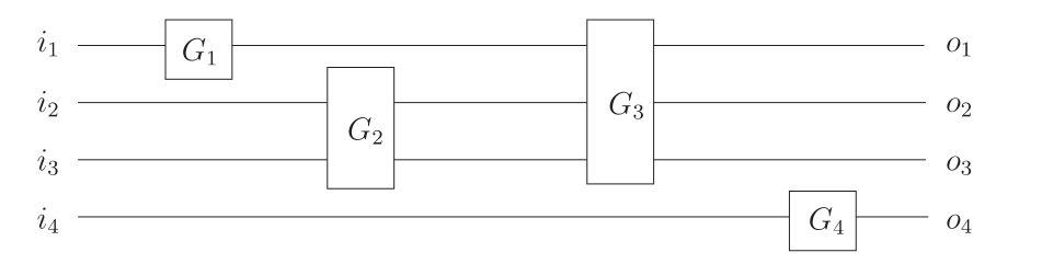
Figure 1. Wires carry the bits and gates.

Quantum computing uses quantum bits (qubits) to process quantum information, A qubit can be \( |0⟩ \) or \( |1⟩ \) , or a superposition of \( |0⟩ \) and \( |1⟩ \) , for example,

\( |ψ⟩=α|0⟩+β|1⟩,\lbrace α,β∈C\rbrace \ \ \ \) (1)

Here, \( |0⟩ \) and \( |1⟩ \) are called ground state, \( α,β \) are plural, they satisfy normalizing condition. Based on equation, we can rewrite the \( |ψ⟩ \) as:

\( |ψ⟩=cos⁡\frac{θ}{2}|0⟩+{e^{iφ}}sin⁡\frac{θ}{2}|1⟩ θ∈[0,π),φ∈[0,2π)\ \ \ \) (2)

\( {e^{iφ}} \) is the relative phase factor. The quantum state can be expressed as a vector on the unit sphere, which is called the Bloch sphere, and its representation in the quantum circuit is shown in Figure 2 [5]. Orthogonal bases \( |0⟩ \) and \( |1⟩ \) representing qubit states are represented by column vectors as:

\( |0⟩=[ \begin{array}{c} 1 \\ 0 \end{array} ],|1⟩=[ \begin{array}{c} 0 \\ 1 \end{array} ]\ \ \ \ \ \ \) (3)

In quantum mechanics, the product between qubits is defined as the tensor product in linear algebra. For example, two qubit states can be written as \( |{ψ_{1}}⟩⊗|{ψ_{2}}⟩ \) , the two qubit states can also be abbreviated as \( |{ψ_{1}}⟩|{ψ_{2}}⟩ \) or \( |{ψ_{1}}{ψ_{2}}⟩ \) . For example:

\( |{ψ_{1}}⟩⊗|{ψ_{2}}⟩=[ \begin{array}{c} {ψ_{10}} \\ {ψ_{11}} \end{array} ]⊗[ \begin{array}{c} {ψ_{20}} \\ {ψ_{21}} \end{array} ]=[ \begin{array}{c} {ψ_{10}}{ψ_{20}} \\ {ψ_{10}}{ψ_{21}} \\ {ψ_{11}}{ψ_{20}} \\ {ψ_{11}}{ψ_{21}} \end{array} ]\ \ \ \) (4)

This can be also be considered as a probabilistic circuit model because quantum physics allows one to understand that the state of a single wire at a given place can be both 0 and 1 with differing probabilities, which is \( ( \begin{array}{c} {p_{0}} \\ {p_{1}} \end{array} ) \) , we write it in Dirac notation:

\( S={p_{0}}|0〉+{p_{1}}|1〉\ \ \ \) (5)

So the probability of combined state of two wires can be written as:

\( ( \begin{array}{c} {p_{0}}{q_{0}} \\ {p_{0}}{q_{1}} \\ {p_{1}}{q_{0}} \\ {p_{1}}{q_{1}} \end{array} )=( \begin{array}{c} {p_{0}} \\ {p_{1}} \end{array} )⊗( \begin{array}{c} {q_{0}} \\ {q_{1}} \end{array} )\ \ \ \) (6)

Here, \( {q_{i}} \) represent the state of probability of the second wires.

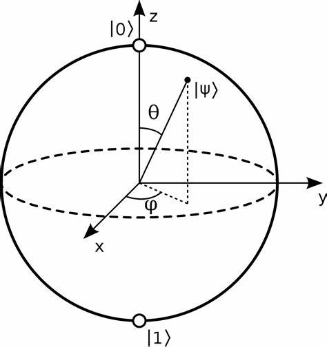
Figure 2. Bloch sphere [5].

2.2. Quantum logic gates

The main role of quantum logic gates is to convert information from one form to another, and in quantum computing, the simplest quantum logic gate is the single qubit gate, which acts on the simplest quantum system. In classical computing, the only non-trivial logic gate is the NOT gate, its function is to exchange 0 and 1. Likewise, in quantum computing, a quantum NOT gate can change state \( α|0⟩+β|1⟩ \) to \( α|1⟩+β|0⟩ \) . We can represent it as a matrix:

\( X=[\begin{matrix}0 & 1 \\ 1 & 0 \\ \end{matrix}]\ \ \ \) (7)

One of the important facts is that The NOT gates are identically the member of Pauli gates:

\( {σ_{0}}≡[\begin{matrix}1 & 0 \\ 0 & 1 \\ \end{matrix}], {{σ_{1}}≡{σ_{x}}≡[\begin{matrix}0 & 1 \\ 1 & 0 \\ \end{matrix}],{σ_{2}}≡{σ_{y}}≡[\begin{matrix}0 & -i \\ i & 0 \\ \end{matrix}],σ_{3}}≡{σ_{z}}≡[\begin{matrix}1 & 0 \\ 0 & -1 \\ \end{matrix}]\ \ \ \) (8)

They are significant because they cover the vector space of operators with a single qubit.

The Hadamard gate is another significant gate. It needs to be considered because algorithms will soon be introduced. The Hadamard gate has the matrix shape depicted below, according to the computational basis:

\( \frac{1}{\sqrt[]{2}}[\begin{matrix}1 & 1 \\ 1 & -1 \\ \end{matrix}]\ \ \ \) (9)

and it has the following properties:

\( H|0〉=\frac{1}{\sqrt[]{2}}(|0〉+|1〉)H|1〉=\frac{1}{\sqrt[]{2}}(|0〉-|1〉)\ \ \ \) (10)

as well as:

\( H={H^{-1}}\ \ \ \) (11)

These important single qubit gates are shown in Figure 3.

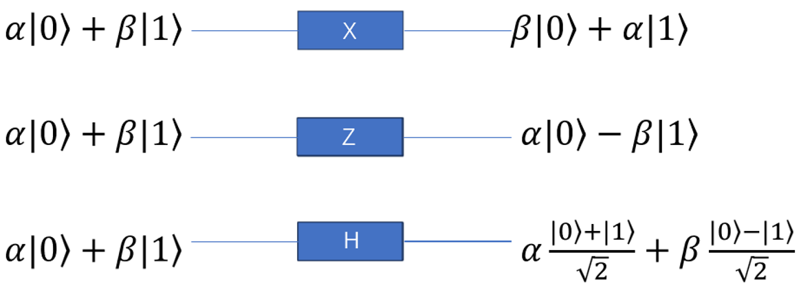
Figure 3. Single qubit gates.

When we input two qubits, the single-quantum logic gate becomes a two-bit quantum gate, such as a controlled NOT gate, and the two input qubits are the control qubit and the target qubit. The function is that when the control qubit is 0, the target qubit will remain unchanged; on the contrary, when the control qubit is 1, the target qubit will be flipped, and the change of the process is as \( |00⟩⟶|00⟩,|01⟩⟶|01⟩,|10⟩⟶|11⟩,|11⟩⟶|10⟩ \) . Likewise, since a controlled NOT gate is also a linear transformation, one can express it in terms of a matrix as and its representation in the quantum circuit can be drawn as Figure 4:

\( CNOT=[\begin{matrix}1 & 0 & 0 & 0 \\ 0 & 1 & 0 & 0 \\ 0 & 0 & 0 & 1 \\ 0 & 0 & 1 & 0 \\ \end{matrix}]\ \ \ \) (12)

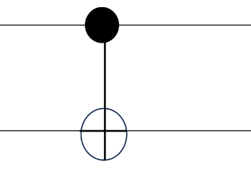
Figure 4. Line representation of controlled NOT gate.

2.3. Quantum parallelism and quantum superposition principle

The quantum state superposition principle shows that if the system can be in the \( |{ψ_{1}}⟩ and |{ψ_{2}}⟩ \) states, then the system can also be in a linear superposition of them \( |ψ⟩=α|{ψ_{1}}⟩+β|{ψ_{2}}⟩ \) . Applying this rule to quantum computing, a qubit can be in state \( |0⟩ \) or state \( |1⟩ \) , it can also be in superposition \( |ψ⟩=α|0⟩+β|1⟩ \) [6]. Quantum parallelism is an essential feature of many quantum algorithms. It is precisely because of this basic characteristic of quantum computing that the values of functions at different values can be calculated simultaneously in a quantum computer

2.4. Quantum entanglement and preparation of quantum entangled state

For a two-qubit system, under certain conditions, if one of the qubits is measured, and then the second qubit is measured, the result obtained is closely related to the measurement result of the first qubit [7]. This correlation is not limited by space. In quantum theory, qubit systems with this property are known as quantum entanglement. Quantum entanglement has been widely used in quantum computing and quantum information, such as quantum teleportation, quantum remote cloning, quantum remote state preparation, etc. Creating entangled states can be achieved through various physical systems, such as atoms, ions, photons, or superconducting circuits. Here are some common methods for creating entangled states: Spontaneous Parametric Down-Conversion (SPDC): This method involves using a nonlinear crystal to generate pairs of entangled photons. When a laser beam passes through the crystal, it can undergo a process called parametric down-conversion, splitting the photons into two entangled photons with correlated properties such as polarization, energy, or momentum; Superconducting Circuits: Superconducting qubits, which are the building blocks of quantum computers, can be used to create entangled states. By applying controlled microwave pulses and exploiting the properties of Josephson junctions, entanglement between multiple qubits can be generated; Ion Traps: In ion trap experiments, individual ions are trapped using electromagnetic fields. By manipulating the internal states of the ions and utilizing the ion's collective motion, entangled states can be created. This technique has been successful in generating entangled states with high fidelity.

3. Quantum computing instruments

Quantum computing is developing rapidly, and all countries have developed advanced quantum computing instruments. The research team of the Chinese Academy of Sciences successfully developed a 62-bit programmable superconducting quantum computing prototype "Zuchongzhi", and realized a programmable two-dimensional quantum walk on this basis. In May 2021, based on "Zuchong No. 1", the research team adopted a brand-new flip-chip 3D packaging process to solve the problem of large-scale bit integration, and successfully developed "Zuchong No. 2", realizing 66 data High-density integration of bits, 110 coupled bits, and 11 channels of reading, the maximum state space dimension reaches 10 to the 19th power. "Zuchongzhi No. 2" can handle the quantum random circuit sampling problem more than 10 million times faster than the current fastest supercomputer [8]. Figure 5 shows the basic structure about this quantum computer.

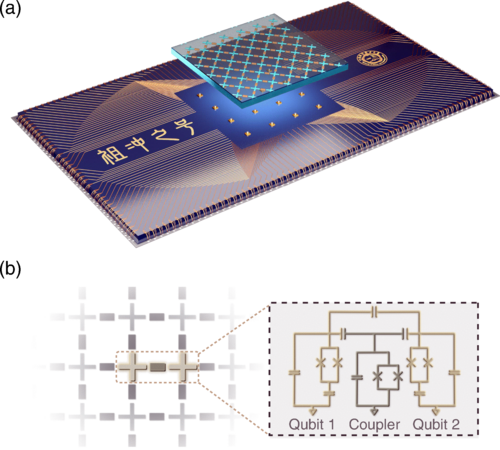
Figure 5. Device schematic of the Zuchongzhi quantum processor. (a) The Zuchongzhi quantum processor consists of two sapphire chips. (b) Simplified circuit schematic of the qubit and coupler [8].

While continuing to develop higher-quality and more scalable optical quantum computing prototypes, Pan Jianwei's team researched applying the Gaussian Bose sampling task performed by "Nine Chapters" to graph theory problems. It is the first to use the Gaussian Bose sampling implemented by "Nine Chapters" to accelerate the solution of graph theory problems by random search algorithm and simulated annealing algorithm. The researchers used more than 200,000 80-photon coincidence counting samples in the experiment, which is about 180 million times faster than the world's fastest supercomputer using the current best classical algorithm to accurately simulate the experiment [9]. In terms of ion trap quantum computers, IonQ has launched a prototype system of ion trap system quantum computers, and its main technical indicators are as follows. As for the number of qubits, up to 160 qubits can be loaded, 79 qubits can perform single-bit operations, and 11 qubits can perform double-bit operations. In terms of programmable quantum computing, 5-bit programmable computing has been realized, and 4 quantum algorithms have been realized on 5 bits [10].

4. Quantum computing algorithm

Although it is challenging to go extensively into a quantum computing algorithm without any prior knowledge of quantum mechanics, cryptography, or mathematics, it is nevertheless possible to grasp the fundamental concepts of the greatest algorithms ever created as quantum computing rapidly gains understanding. Several algorithms will be discussed in more generic terms in the content that follows rather than being rigorously proved.

4.1. The advantage of quantum algorithm

The Deutsch Algorithm is the first algorithm this post would like to introduce. Despite being quite old, it nevertheless supports modern algorithms and reveals the core parallelism of quantum computing [4]. Given an unknown 1-bit function \( f \) that maps \( \lbrace 0,1\rbrace \) to \( \lbrace 0,1\rbrace \) , Deutsch wants to figure out what it is \( f(0)⊕f(1) \) . the symbol \( ⊕ \) means ‘XOR’, which means: \( f(0)⊕f(1)=1,f(0)≠f(1) \) while \( f(0)⊕f(1)=0,f(0)=f(1) \) . The algorithm wins its advantages that it only needs one time to make a query to determine the value of \( f(0)⊕f(1) \) ,comparing with the classical algorithm that need to get both values of and \( f(1) \) . Here comes with the algorithm. One defines a Unitary operator:

\( {U_{f}}:|x〉|y〉↦|x〉|y⊕f(x)〉\ \ \ \) (13)

and sets \( |y⟩=|0⟩ \) ,and \( |x⟩=\frac{1}{\sqrt[]{2}}|0⟩+\frac{1}{\sqrt[]{2}}|1⟩ \) , Input them into the circuit and operate \( {U_{f}} \) on it:

\( {U_{f}}(\frac{1}{\sqrt[]{2}}|0〉+\frac{1}{\sqrt[]{2}}|1〉)|0〉=\frac{1}{\sqrt[]{2}}{U_{f}}|0〉|0〉+\frac{1}{\sqrt[]{2}}{U_{f}}|1〉|0〉=\frac{1}{\sqrt[]{2}}|0〉|f(0)〉+\frac{1}{\sqrt[]{2}}|1〉|0⊕f(0)〉\ \ \ \) (14)

If the initial state is set with:

\( |{ψ_{0}}〉=|0〉(\frac{1}{\sqrt[]{2}}(|0〉-|1〉))\ \ \ \) (15)

First it needs to be applied with the Hadamard gate (equation 10):

\( H|{ψ_{1}}〉=\frac{1}{\sqrt[]{2}}(|0〉+|1〉)(\frac{|0〉-|1〉}{\sqrt[]{2}})\ \ \ \) (16)

Then if apply the unitary gate on it (equation 13):

\( {U_{f}}(H|{ψ_{1}}〉)={(-1)^{f(0)}}(\frac{|0〉+{(-1)^{f(0)⊕f(1)}}|1〉}{\sqrt[]{2}})(\frac{|0〉-|1〉}{\sqrt[]{2}})\ \ \ \) (17)

By using the inverse Hadamard again, it could be notified that if \( f(0)⊕f(1)=0 \) , the result will be:

\( {(-1)^{f(0)}}|0〉(\frac{|0〉-|1〉}{\sqrt[]{2}})\ \ \ \) (18)

However, if \( f(0)⊕f(1)=1 \) ,the result is changed to:

\( {(-1)^{f(0)}}|1〉(\frac{|0〉-|1〉}{\sqrt[]{2}})\ \ \ \) (19)

The Deutsch Algorithm shows that it only needs one query to get \( f(0)⊕f(1) \) !

4.2. Shor find order and realization

Another algorithm that has achieve great success is Shor’s algorithm. It is used to factor large integral N especially for RSA encryption which postulate that the factoring of large numbers is exponentially harder. Whereas, with Shor’s algorithm, this operation could be done in polynomial time. One might briefly summarize Shor's algorithm by utilizing the ability of quantum computing's linear combinations of states to collapse the states in order to identify the order of [11]:

\( f(x)=f(x+r)={a^{x}}modN\ \ \ \) (20)

which could be transform to:

\( {a^{x}}={a^{x+r}}(mod N) \)

\( {a^{r}}=1(mod N) \)

\( ({a^{\frac{r}{2}}}+1)({a^{\frac{r}{2}}}-1)=kN(k=0,1,2,\cdot \cdot \cdot )\ \ \ \) (21)

If using Euclidean algorithm (Knuth, 1981), The two dividers of 𝑁 thus obtained. The goal of Shor’s algorithm is to finding \( r \) , especially using phase estimation to give the order of \( f(x) \) . To understand how Shor’s algorithm work, the fundamental knowledge of phase estimation is presented here. Fourier transform is known as a good method to decompose an input and represent the signal in its phase space. The Fourier transform and inverse transform of an eigenstates \( |x〉 \) is defined as following [12]:

\( QFT|x〉=\frac{1}{\sqrt[]{{2^{n}}}}\sum _{y=0}^{{2^{n}}-1}{e^{2πi\frac{x}{{2^{n}}}y}}|y〉\ \ \ \) (22)

\( QF{T^{-1}}\frac{1}{\sqrt[]{{2^{n}}}}\sum _{y=0}^{{2^{n}}-1}{e^{2πi\frac{x}{{2^{n}}}y}}|y〉=|x〉\ \ \ \) (23)

As an application of Fourier transform, phase estimation could be briefly proved by following steps. One supposes there is a unitary operator:

\( {U_{a}}:|s〉↦|sa mod N⟩ ,0⩽s \lt N\ \ \ \) (24)

Since equation (21), The \( r \) th operation of a unitary operator form a period to get back \( |s〉 \) :

\( U_{a}^{r}:|s〉↦|s{a^{r}} mod N〉=|s〉\ \ \ \) (25)

A Unitary operator can have its eigenvalues which should be the \( r \) th roots of 1 if operator satisfied the above properties. Considering a state \( |{φ_{k}}〉 \) in terms of following form:

\( |{φ_{k}}〉=\frac{1}{\sqrt[]{r}}\sum _{s=0}^{r-1}{e^{-2πi\frac{k}{r}s}}|{a^{s}}mod N〉\ \ \ \) (26)

Applying the unitary operator then the phase could be isolated:

\( {U_{a}}:|{φ_{k}}〉=\frac{1}{\sqrt[]{r}}\sum _{s=0}^{r-1}{e^{-2πi\frac{k}{r}s}}{U_{a}}|{a^{s}}mod N〉={e^{2πi\frac{k}{r}}}|{φ_{k}}〉\ \ \ \) (27)

With the property listed above, here is the solution of finding an order of Random integer multiple of \( \frac{1}{r} \) [4]. Let the Input parameter contains two registers, one is control register and another is target register and they are entangled.

\( |{ψ_{0}}〉=\sum _{x=0}^{{2^{n}}-1}\frac{1}{\sqrt[]{{2^{n}}}}|x〉|{a^{x}}mod N〉\ \ \ \) (28)

With the Fourier transform being applied and rewrite it as:

\( |{ψ_{0}}〉=\sum _{b=0}^{r-1}\frac{1}{\sqrt[]{{2^{n}}}}(|x〉\sum _{z=0}^{{m_{b}}-1}|zr+b〉)|{a^{b}}mod N〉\ \ \ \) (29)

Where \( {m_{b}} \) should satisfy: \( ({m_{b}}-1)r+b⩽{2^{n}}-1 \) to get enough bits. Measuring the second register will cause the first register collapse to the superposition of:

\( \frac{1}{\sqrt[]{{m_{b}}}}\sum _{z=0}^{{m_{b}}-1}|zr+b〉\ \ \ \) (30)

Finally, by using inverse QFT to get:

\( \sum _{j=0}^{{m_{b}}-1}{e^{-2πi\frac{b}{r}s}}|{m_{b}}j〉\ \ \ \) (31)

The measure value of the first register should be \( x={m_{b}}j \) ,since the \( r \) and \( j \) is unknown, it should use \( QFT_{{2^{n}}}^{-1} \) to get the approximate phase term, then output will give us the weighted mixture of the states of \( |\widetilde{k/r}〉 \) for some \( k∈\lbrace 0,1,...,r-1\rbrace \) . And with the estimation of \( \frac{x}{{2^{n}}}≈\frac{k}{r} \) , it could be finally evaluated by continued fractions algorithm. Figure 6 has demonstrate the basic realization of Shor’s algorithm.

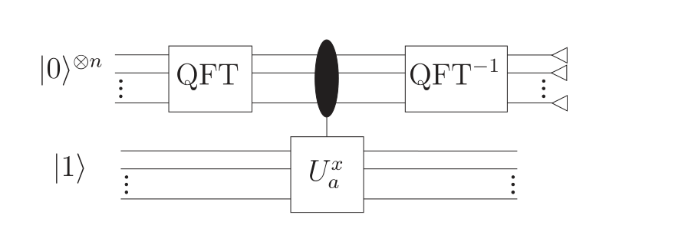
Figure 6. The demonstration of circuit of basis phase estimation [4].

4.3. Distributed Shor’s algorithm

Despite the Shor algorithm's great success, the original Shor’s algorithm is based on a centralized architecture in which all of the qubits are concentrated in one place. This is not practical for large-scale factorization problems that require a large number of qubits. Shor’s algorithm needs the \( 2L+O(1) \) bits to perform when factoring L-bit integer. The distributed architecture-specific Shor's algorithm is a variant of the original Shor's algorithm. The central notion of distributed quantum Shor's algorithm divides the quantum registers among numerous network nodes and uses a distributed protocol to carry out the quantum operations. With this method, the factorization problem may be divided into smaller issues that can be resolved in parallel, which can drastically cut down on the amount of time needed for factorization. Yimsiriwattana developed the first distributed methods in 2004. They separated the quantum circuit and built-up global quantum gates for communication, although the complexity is high to \( O({L^{2}}) \) [12]. Another research by Teams of Xiao et al. proposed a distributed quantum classical hybrid order-finding algorithm that reduce the complexity to \( (1-\frac{1}{k})L-lo{g_{2}}k \) using \( k \) computers and each been signed to factor partial of the total bits, and the complexity of it is \( O(kL) \) [13]. For the realization of the algorithm, they divided the estimation into the first \( \frac{L}{2}+1 \) bits on the computer A and then the \( \frac{L}{2}+2th \) bit to the \( (2L+1) \) th bit on computer B. By the definition a new unitary Matrix:

\( {M_{a}}|x〉=|ax mod N〉\ \ \ \) (32)

\( {M_{a}}|{u_{s}}〉={e^{2πi\frac{s}{r}}}|{u_{s}}〉\ \ \ \) (33)

And a controller operator \( {C_{m}}({M_{a}}) \) to perform operation on the second register:

\( {C_{m}}({M_{a}})|j〉|x〉=|j〉|{a^{j}}x mod N〉\ \ \ \) (34)

Then by using \( M_{a}^{{2^{l}}}|{u_{k}}〉 \) :

\( M_{a}^{{2^{l}}}|{u_{k}}〉={e^{2πi({2^{l}}\frac{k}{r})}}|{u_{k}}〉\ \ \ \) (35)

and as well as \( {C_{t}}(M_{a}^{{2^{l}}}) \) ,they realize the division of work with quantum teleportation between two computers. note that in equation (35), if a phase \( ω \) is defined as [10]:

\( \frac{k}{r}=ω=0.{x_{1}}{x_{2}}{x_{3}}\cdot \cdot \cdot \ \ \ \) (36)

There is:

\( {2^{l}}\frac{k}{r}={x_{1}}{x_{2}}{x_{3}}\cdot \cdot \cdot {x_{k}}.{x_{k+1}}{x_{k+2}}\cdot \cdot \cdot \ \ \ \) (37)

For any integer \( l \) , \( {e^{2πi{2^{l}}}}=1, \) It could be obtained that:

\( {e^{2πi({2^{l}}\frac{k}{r})}}={e^{2πi(0.{x_{k+1}}{x_{k+2}}\cdot \cdot \cdot )}}\ \ \ \) (38)

Finally, the results of two computers should be combined to obtain the correct \( r \) . With this approach, the mistake has been decreased and computer bits have been preserved. The work of Fleury and Lacomme has been used to demonstrate another variant of Shor's algorithm in IBM's quantum physical optimizers [14]. They have created a method for evaluating the order of an indirectly. They alter the order of the element which supposed in the group of multiplication ( \( mod N \) ) to the computation of the phase additive group ( \( mod 2π \) ). By changing the

\( {U_{f}}|x〉⊗|y〉=|x〉⊗|y⊕{a^{l}}mod N〉\ \ \ \) (39)

which can be obtained by equation (13)

\( U_{N}^{{ψ_{a}}}|x〉⊗|y〉=|x〉⊗|y⊕{ψ_{{a^{l}}}}mod 2π〉\ \ \ \) (40)

With the definition of:

\( {ψ_{a}}=\frac{2.π}{N}.a\ \ \ \) (41)

\( {ψ_{{a^{{2^{j}}}}}}=({2^{j-1}}mod N).\frac{2.π}{N}.a\ \ \ \) (42)

With a several step’s calculation, the property of \( {ψ_{{a^{{2^{p}}}}}} \) is:

\( {ψ_{{a^{{2^{p}}}}}}={ψ_{{a^{{2^{p}}-1}}}}+\sum _{k=1}^{{2^{p-1}}}{ψ_{a}}={ψ_{{a^{{2^{p}}-1}}}}+{2^{p-1}}.{ψ_{a}}\ \ \ \) (43)

The \( j \) th qubit \( |ψ_{{a^{k}}}^{j}〉 \) of \( |ψ_{{a^{k}}}〉 \) might be acquired in the end by using the \( U_{N}^{{ψ_{a}}} \) according to the same process as in Figure 5:

\( |ψ_{{a^{k}}}^{j}〉=\frac{1}{2}(|0〉+{e^{2.π.i.\frac{b}{{2^{j}}}}}|1〉)\ \ \ \) (44)

This method demonstrates efficiency in terms of qubits and gates, and it has already been successfully tested on a physical quantum optimizer using an experiment with an integer size of more than 100 bits. With the ceaseless efforts of scientists and researchers, Quantum algorithm shows promising future and potential to solve more problems. Although it hasn’t been proved yet that quantum computing could solve problems complex as NP, but it contains vitality and flexibility. And last but not least, the creativity and physical verification is vital.

5. Applications

Quantum computing has the potential to revolutionize various fields by solving complex problems more efficiently than classical computers. Quantum computing can tackle optimization problems, such as finding the most efficient routes for delivery or minimizing operational costs. It can provide solutions for resource allocation, supply chain optimization, and scheduling optimization. In addition, quantum simulations can help in accelerating the discovery of new drugs by analysing molecular interactions and simulating complex biological systems. Quantum computing can also assist in designing new materials with specific properties by modelling their atomic and molecular behaviour. Existing drug discovery systems can perform hundreds of millions of comparisons for molecules of a given size with the help of classical computers. Quantum computers can map trillions of molecular compositions and quickly identify the most effective combinations among them. By comparing macromolecules, they can further advance the treatment of various diseases with medical products [15]. Moreover, quantum computing can improve financial modelling and risk assessment by efficiently handling large datasets and complex calculations. It can contribute to portfolio optimization, options pricing, risk analysis, and fraud detection. Besides, quantum computing has implications for cryptography as it can potentially break some of the widely used cryptographic algorithms. On the other hand, quantum cryptography offers secure communication based on the principles of quantum mechanics. Furthermore, quantum computing can simulate molecular interactions accurately, aiding in the study of chemical reactions, catalyst design, and drug discovery. In 2017, IBM used the variational quantum eigen solution algorithm (VQE) on its superconducting quantum computer (6 qubits) to achieve an accurate calculation of the ground state energy of beryllium hydride (BeH2) molecules. In 2020, the Google quantum team used the VQE algorithm to successfully simulate the isomerization reaction process and binding energy of diazene molecules on its Sycamore quantum processor (12 qubits), which can achieve accurate calculation and analysis of electronic structures and chemical reactions. It is currently the largest-scale chemical reaction simulation calculation realized by quantum computers. In 2021, the IBM quantum computing team shortened the modelling time of lithium hydride (LiH) chemical molecules to 9 hours and increased the speed by 120 times through comprehensive optimization of quantum algorithms, system software, processors, and control systems, thereby maximizing the use of computing power. time, minimize waiting time [16].

6. Discussion

While quantum computing holds great promise, several limitations and challenges need to be addressed. Quantum states are highly sensitive to noise, interference, and environmental disturbances. Maintaining and controlling the fragile quantum states, known as qubits, is challenging due to the phenomenon of decoherence. Errors can occur during computation, limiting the accuracy and reliability of results. Scaling up the number of qubits while maintaining their coherence is a significant challenge. It is crucial to increase qubit counts to perform complex calculations and achieve a practical quantum advantage. However, as the number of qubits increases, so does the susceptibility to noise and errors. Quantum error correction is crucial for fault-tolerant quantum computing. Implementing error correction codes requires additional qubits and more computational resources, making the systems more complex and demanding. Quantum operations, such as gates, need to be precise and well-controlled. However, not all desired quantum operations are easy to implement. Certain interactions between qubits may be inherently difficult or even impossible to achieve, limiting the range of computations that can be performed. Coherence time refers to the duration during which qubits maintain their quantum state before decoherence occurs. Coherence times are relatively short compared to the time required for complex calculations. Prolonging coherence times is crucial for performing lengthy computations. Building and maintaining quantum hardware with low error rates is a significant challenge. Current technologies, such as superconducting circuits or ion traps, require sophisticated and expensive infrastructure, cryogenic temperatures, and complex control systems. Quantum algorithms often require a large number of operations and qubits to achieve meaningful results. Implementing and executing these algorithms can be resource-intensive and computationally demanding.

The field of quantum computing is still in its early stages, and there are many exciting prospects for future research. First, consider increasing the fault tolerance of quantum computing. Developing robust error correction techniques and fault-tolerant quantum computing methods is crucial to overcome the limitations of noise and decoherence. Research is ongoing to design and implement efficient error-correcting codes, quantum error mitigation strategies, and fault-tolerant architectures. In addition to reducing error rates, understanding the sources and characteristics of errors in quantum systems is also crucial for error mitigation. The research aims to develop techniques for describing and mitigating errors, including error models, error detection methods, and error suppression algorithms. To increase computing power, it is possible to expand the number of qubits and build larger, more complex quantum systems. The number of qubits in a system can be increased by improving qubit consistency, reducing error rates and developing new methods. In terms of algorithms and programs, research can focus on designing efficient algorithms for optimization problems, machine learning, cryptography, and simulating quantum systems. Quantum simulator is also one of the research hotspots. Quantum simulators provide insight into complex quantum systems to solve problems in materials science, chemistry and condensed matter physics. Furthermore, exploring the synergy between classical and quantum computing is an active research area. Combining classical and quantum algorithms to solve complex problems (known as hybrid computing) can take advantage of the strengths of both systems and overcome the limitations of quantum computing alone. Quantum communication is also a very important research direction. Research in this area focuses on quantum key distribution, quantum repeaters and quantum networks to enable large-scale quantum communication. As quantum computing advances, interdisciplinary collaborations among physicists, computer scientists, mathematicians, and engineers will continue to drive research and innovation in this field. The future holds enormous potential for breakthroughs that will shape the computing landscape and revolutionize industries.

7. Conclusion

Due to its excellent computing power, quantum computers can solve many problems that traditional computers cannot solve, and algorithms are one of the keys to improving computing power. This study first introduces the basic principles of quantum computing, e.g., qubits, quantum gates, quantum entanglement and the preparation of entangled states. Afterwards, this article selects some advanced quantum computing instruments, such as Zu Chongzhi, to introduce their basic parameters and achievements. Then this article begins to explain the quantum computing algorithm, focusing on the modern realization of Shor algorithm, reflecting the efficiency and distinction of quantum computing algorithms compares with the traditional computers. The quantum computing algorithm focus on solving the problems within polynomial time. This paper also introduces the application of quantum computing in some fields (medicine, finance, chemistry, etc.), and shows the broad application prospects of quantum computing. Finally, this paper points out some shortcomings of current quantum computing from the perspectives of security, energy consumption, stability, etc., and gives specific goals for future development. This article summarizes the important applications and key algorithms of quantum computing in recent years, aiming to help future generations learn quantum computing.

Authors contribution

All the authors contributed equally and their names were listed in alphabetical order.

References

[1]. Xing D 2020 China New Communications vol 19 pp 64-65.
[2]. Wu Y 2023 Nature Magazine vol 01 p 32+44.
[3]. Wu C 2021 Science and Technology Daily, vol 10-27 p 003.
[4]. Kaye P, Laflamme R and Mosca M 2006 An introduction to quantum computing (OUP Oxford).
[5]. Ji W 2022 Quantum computing simulation of quantum dynamical system and its characteristics research (Master's thesis, China University of Mining and Technology).
[6]. Liu S 2012 Realization of Set Operations on Quantum Computer (Master's Thesis, Sichuan Normal University).
[7]. Simon S H, Bonesteel N E, Freedman M H, Petrovic N and Hormozi L 2006 Physical Review Letters vol 96(7) p 070503.
[8]. Wu Y, Bao W S, Cao S et al. 2021 Physical Review Letters vol 127(18), p 180501
[9]. Xu H 2021 Henan Science and Technology vol 31 p 1.
[10]. Long G 2021 People's Forum Academic Frontiers vol 07 pp 44-56.
[11]. Shor P W 1999 SIAM review vol 41(2) pp 303-332.
[12]. Xiao L, Qiu D, Luo L and Mateus P 2023 ArXiv preprint arXiv:2304.12100.
[13]. Yimsiriwattana A and Lomonaco S J 2004 Quantum Information and Computation II, vol 5436.
[14]. Gérard F and Lacomme P 2022 A technical note for a shor's algorithm by phase estimation (Tech Science Press).
[15]. Chen C, Xing H and Tan D 2022 China Digital Medicine vol 12 pp 34-39.
[16]. Zhu W, Wang K, Xu D, Wu L and Cheng Y 2022 Frontiers of Data and Computing Development vol 02, pp 131-140.
Cite this article
Yang,R.;Zhong,Z. (2023). Algorithm efficiency and hybrid applications of quantum computing. Theoretical and Natural Science,11,280-290.
Data availability
The datasets used and/or analyzed during the current study will be available from the authors upon reasonable request.
Disclaimer/Publisher's Note
The statements, opinions and data contained in all publications are solely those of the individual author(s) and contributor(s) and not of EWA Publishing and/or the editor(s). EWA Publishing and/or the editor(s) disclaim responsibility for any injury to people or property resulting from any ideas, methods, instructions or products referred to in the content.
About volume
Volume title: Proceedings of the 2023 International Conference on Mathematical Physics and Computational Simulation
© 2024 by the author(s). Licensee EWA Publishing, Oxford, UK. This article is an open access article distributed under the terms and
conditions of the Creative Commons Attribution (CC BY) license. Authors who
publish this series agree to the following terms:
1. Authors retain copyright and grant the series right of first publication with the work simultaneously licensed under a Creative Commons
Attribution License that allows others to share the work with an acknowledgment of the work's authorship and initial publication in this
series.
2. Authors are able to enter into separate, additional contractual arrangements for the non-exclusive distribution of the series's published
version of the work (e.g., post it to an institutional repository or publish it in a book), with an acknowledgment of its initial
publication in this series.
3. Authors are permitted and encouraged to post their work online (e.g., in institutional repositories or on their website) prior to and
during the submission process, as it can lead to productive exchanges, as well as earlier and greater citation of published work (See
Open access policy for details).