1. Introduction

The research on turbulence models and their applications in wind tunnels has always been a hot topic of research and development. Accurately understanding and predicting the turbulence characteristics of wind tunnels is of great significance in Aeronautics, Automotive design and aerodynamic construction. Over the years, significant progress has been made in the development of turbulence models, and computational fluid dynamics (CFD) has become the main choice for exploring the flow forms of wind tunnels and other fluids [1]. Computational fluid dynamics (CFD) is used to study and analyze air flow characteristics and temperature distribution [2].

This article focuses on the performance of several turbulence models in wind tunnel experiments. The specific issue that needs to be addressed is to compare and evaluate various turbulence models in tunnel airflow simulation. By comparing the results of these models, the purpose of this article is to determine the advantages and disadvantages of each model and understand their applicability in simulated wind tunnels.

To achieve this objective, a combination of numerical simulation methods and experimental data will be utilized. CFD techniques will be employed to create numerical models of wind tunnel configurations and apply different turbulence models for simulating the turbulent flow. The simulated results will be compared with experimental data obtained from wind tunnel tests to assess the accuracy and performance of each turbulence model.

The significance of this research lies in its potential to enhance the understanding and application of turbulence modeling in wind tunnel experiments. By systematically evaluating and comparing various turbulence models, this study will contribute to improving the reliability and accuracy of wind tunnel simulations. The findings can aid researchers, engineers, and designers in selecting appropriate turbulence models for their specific wind tunnel experiments, leading to more precise and efficient aerodynamic analyses. Furthermore, the insights gained from this research can contribute to the development and advancement of turbulence modeling techniques in general, benefiting the broader field of fluid dynamics.

2. Turbulence models

Turbulence models can be divided into two categories: Reynolds-Averaged Navier-Stokes (RANS) models and Large Eddy Simulation (LES). RANS models average the turbulent flow variables over time and decompose them into mean and fluctuating components to solve the mean equations. Common RANS models include the k-ε model, k-ω model, and RNG k-ε model. These models are based on different assumptions and equations to describe shear stress, turbulent energy transfer, and turbulence dissipation.

The Les model directly simulates eddy currents by dividing the flow field into large and small regions. In this article, large-scale turbulent structures are the maintenance of numerical methods for simulating or solving small-scale turbulence. The Rice model can provide more detailed interference information, but the cost calculation is higher. They are suitable for large Reynolds disturbances and large influx.

2.1. Standard k-ε turbulence model

The purpose of the k-ε model is to simulate and predict the turbulent kinetic energy and turbulent dissipation rate in turbulent flows. It purposed is to predict airflow away from wall or surface [3, 4]. According to the Boussinesq hypothesis written in Eq. (1) [1].

\( \frac{∂(ρk)}{∂t}+\frac{∂(ρuk)}{∂xi}=\frac{∂}{∂xj}[(μ+μt)(\frac{∂uk}{∂xj})]+ Pk + Pb - ρε + YM + Sk \) (1)

2.2. Standard k-ω model

The equations governing the turbulence kinetic energy and specific dissipation rate are [5],

\( \frac{∂(ρk)}{∂t}+\frac{∂(ρkuj)}{∂xj}=\frac{∂}{∂xj}[(μ+\frac{μt}{{δ_{k}}})(\frac{∂k}{∂xj})]+ Pk + Pb - ρε + YM + Sk \) (2)

Turbulent kinetic energy and the rate of dissipation are certainly written in the form of Eq. (2).

2.3. RSM model

The RSM model considers the anisotropic nature of turbulence and provides more detailed information about the turbulence structure compared to other models. However, it's important to note that the RSM model has certain limitations. It requires accurate and detailed boundary conditions, as well as appropriate mesh resolution to capture the turbulence scales of interest. The RSM model is computationally expensive compared to simpler models like the k-ε or k-ω models. The equation as [6]:

\( \frac{∂}{∂{x_{k}}}(ρ{u_{k}}\bar{u_{i}^{`}u_{j}^{`}})=\frac{∂}{∂{x_{k}}}(\frac{{u_{k}}}{{σ_{k}}} \frac{∂\bar{u_{i}^{`}u_{j}^{`}}}{∂{x_{k}}})+\frac{∂}{∂{x_{k}}}[μ\frac{∂}{{x_{k}}}(\bar{u_{i}^{`}u_{j}^{`}})]-ρ(\bar{u_{i}^{`}u_{j}^{`}}\frac{∂{u_{j}}}{∂{x_{k{P_{ij}}}}}+\bar{u_{i}^{`}u_{j}^{`}}\frac{∂{u_{i}}}{∂{x_{k}}})+{Φ_{ij}}-\frac{2}{3}{σ_{ij}}ρε \) (3)

2.4. SST k-ω model

The SST k-x model (Eq. (4)) tends to model turbulence near the wall as a consequence of the friction between the fluid and the field it passes at the high price of the Reynolds number [1].

\( \frac{∂(ρω)}{∂t}+\frac{∂(ρω{u_{i}})}{∂{x_{i}}}=\frac{∂}{∂t}({Γ_{ω}}\frac{∂ω}{∂{x_{j}}})+{G_{ω}}-{Y_{ω}}+{D_{ω}}+{S_{ω}} \) (4)

2.5. LES model

This model is suitable for simulating turbulent flow in various structures, especially in the case of a large number of Reynolds numbers. The Les model aims to directly simulate large-scale turbulent structures, while using methods similar to small structures to provide more accurate turbulence predictions. Calculate according to equation 5 and SGS viscosity [1].

\( \frac{∂{\bar{u}_{i}}}{∂t}+\frac{∂\bar{{u_{i}}}\bar{{u_{j}}}}{∂{x_{j}}}={δ_{li}}-\frac{\frac{1}{ρ}∂\bar{p}}{∂\bar{{x_{i}}}}+∂/∂\bar{{x_{i}}}[\frac{∂\bar{{u_{i}}}}{∂{x_{j}}}(v+{v_{T}})] \) (5)

3. CFD method

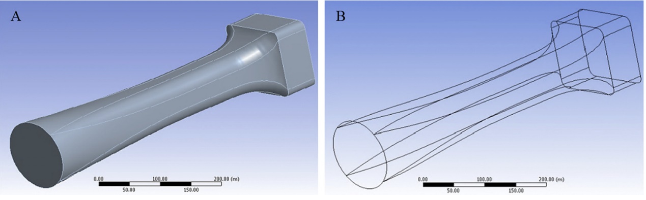
Figure 1. Wind tunnel by ANSYS® 15.0 [1].

Figure 1 is a wind tunnel model. Different disease models have different standards and assumptions. Standard k-ε, k-ω, SST k-ω, RSM models, for instance, It is very important to select and adjust model parameters correctly to adapt to specific traffic conditions. For me, a suitable network model and necessary filtering metrics. Like the motion model, it flows with the recovery of areas that may rise in the simulation [7]. It is crucial to select and adjust appropriate model parameters when simulating the flow during regional recovery. During the process of regional restoration, it may be necessary to adjust the parameters of the RSM model to adapt to specific traffic conditions.

Boundary conditions: Correct adjustment of boundary conditions is crucial for the accuracy of model results. It is important to understand the boundary conditions required for each turbulence model and make corresponding adjustments according to the requirements of the model. Especially for flows with wall edges, the applicability of wall functions and Boundary layer modeling methods must be considered.

Due to limitations in conditions, this article directly uses bibliographic data for analysis.

4. Results and discussion

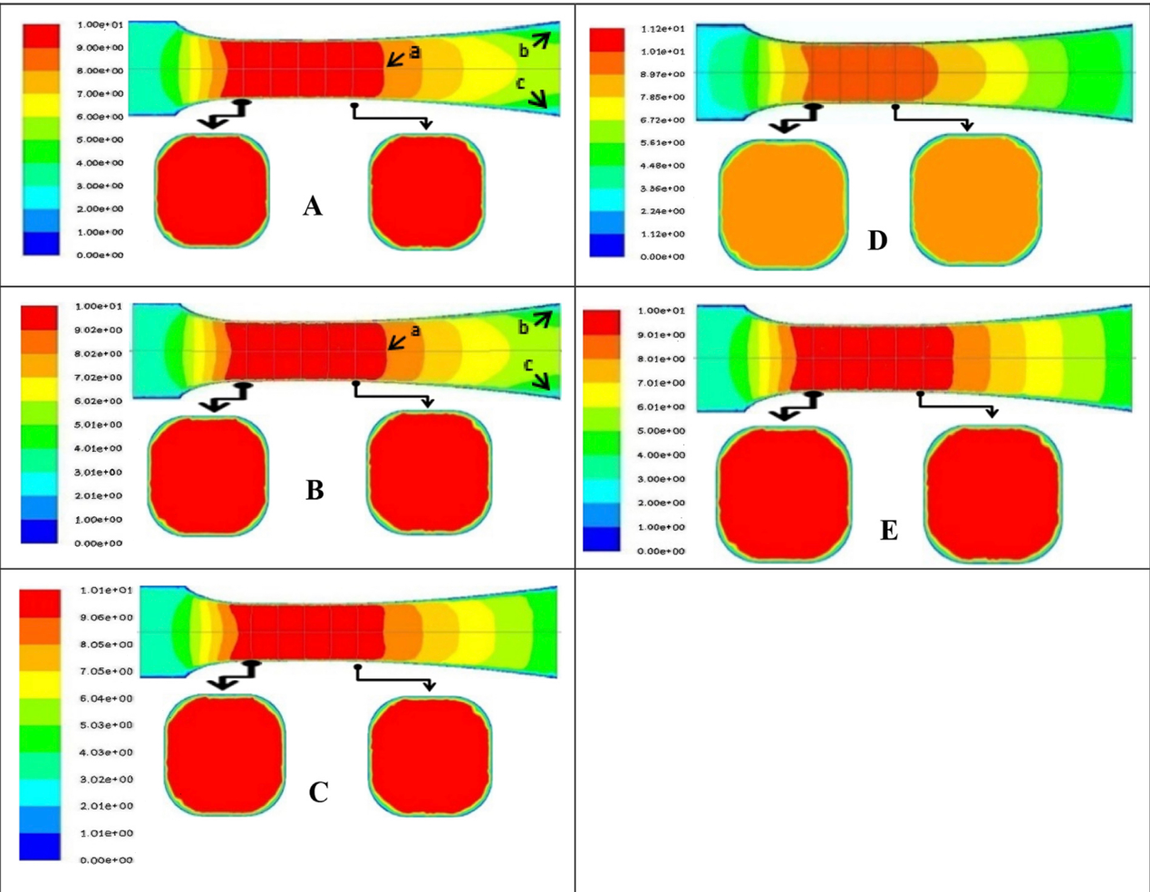
Figure 2. The sequential velocity distribution of each model k-ε (a), k-ω (b), RSM (c), SST k-ω (d), LES (e) at U0 = 3.3m/s [1].

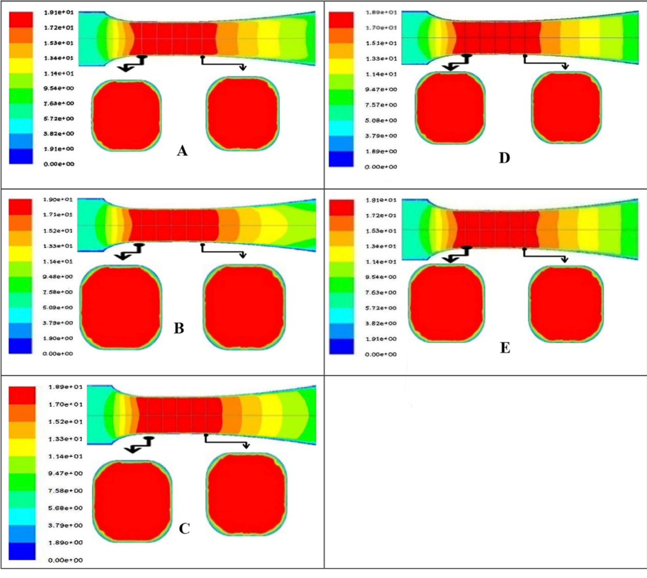
Figure 3. The sequential speed distribution of each model k-ε (a), k-ω (b), RSM (c), SST k-ω (d), LES (e) at U0 = 6.6 m/s [1].

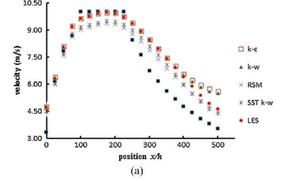
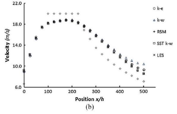
Figure 4. Graphic U0 = 3.3 m/s (a) and U0 = 6.6 m/s (b) of fifth turbulence models [1].

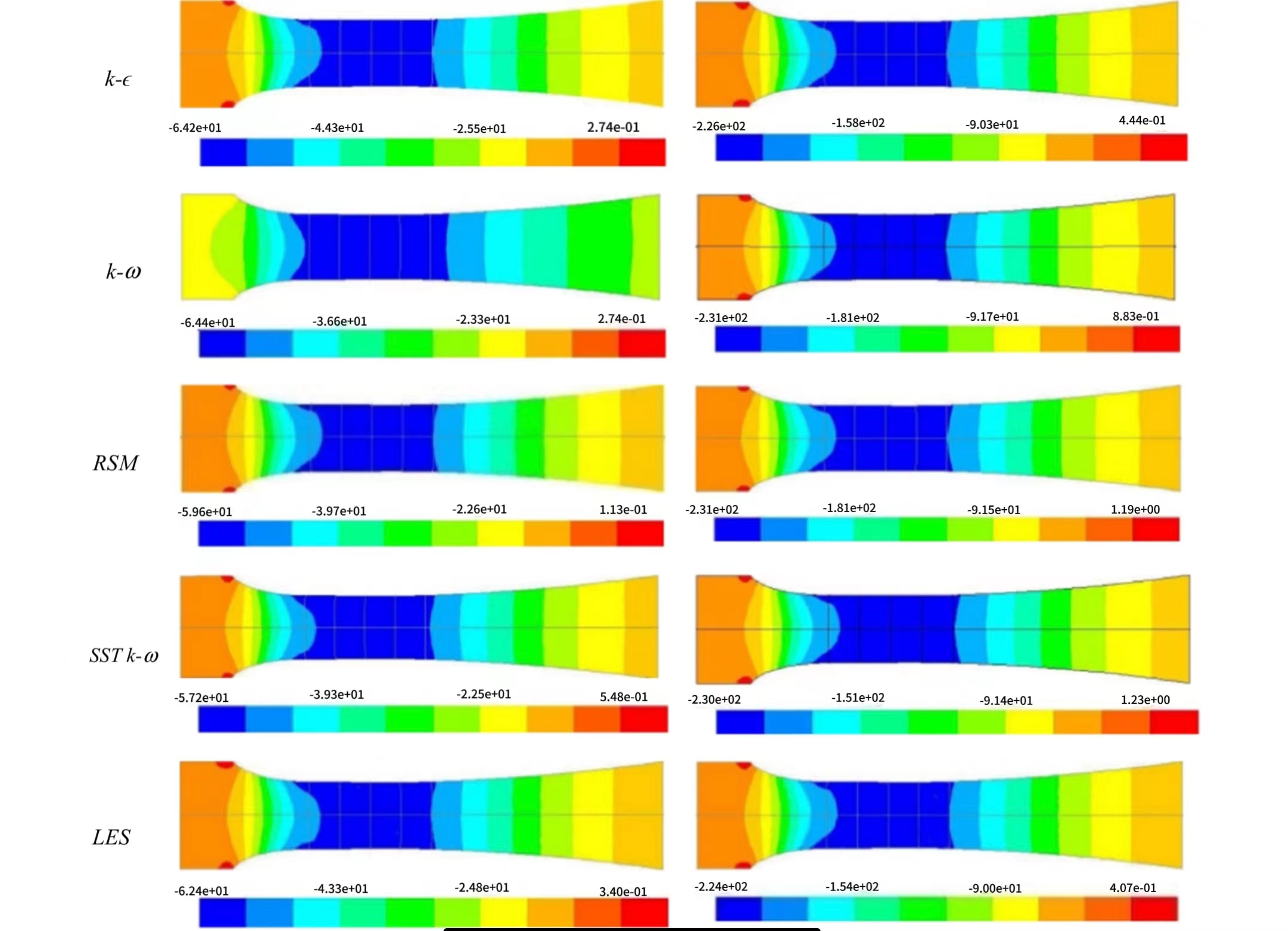
Figure 5. Pressure distribution at U0 = 3.3 m/s (a) and U0 = 6.6 m/s (b) [1].

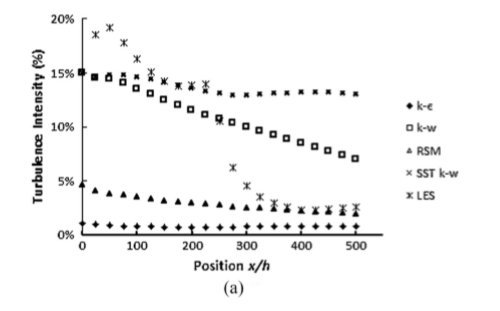
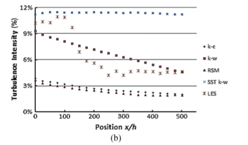
Figure 6. Turbulence Intensity Chart of five turbulence models on U = 10 m/s (a) dan U= 20 m/s (b) [1].

Previous research on wind tunnel experiments mainly focused on the implementation of wind tunnel plans [7-8]. There are also comments on wind tunnels, but they only provide a general description of the airflow [9].

As shown in Figures 2-3, different turbulence models in the experimental section display different velocity profiles. In addition, the velocity distribution determined in the test section varies with different initial velocities. The arrows in Figures 2-3 indicate the bending direction towards the experimental area due to axial flow and the inclined wall of the diffuser. When entering the testing section, all models will be tested for this recovery process. At an initial speed of 3.3 Metre per second, the design speed of the wind tunnel test section is about 10 Metre per second. Under laboratory conditions, the velocity of liquids is estimated to be 10-20 meters per second. Among these five CFD models, the average wind tunnel speed of the K-EPSILON and K-Omega models is 10 m/s.

Figure 5 shows the distribution of five fluid electrostatic turbulence models with initial velocities of 3 m/s and 6 m/s in a wind tunnel. The blue gradient represents the minimum pressure in the wind tunnel, while the red gradient represents the maximum pressure. Although there were different pressure distributions in the five turbulence models, it was observed that the pressure decreased with the airflow in the test area and then increased as the airflow left the test area.

The description of wind tunnel pressure dispersion is consistent with that of Ahmed D.E. et al. Article [10] only uses half of the wind tunnel profile.

Figure 6 shows the turbulence intensity of five turbulence models, while the velocity profile in Figure 4 shows the highest velocity and tends to be smooth. These five CFD models have different turbulence intensities. The LES model has the maximum tilt, while the turbulence of the other four models is relatively flat. Figure 6 shows the turbulence intensity of each model at 10 meters/second or 20 meters/second. The turbulence range of the LES model is 5% to 11%, the K-EPSON model is 2.6% to 3.2%, the K-Omega model is 7% to 8%, and the RSM model is 2.3% to 2.9%, which is very close to the K model.

5. Conclusion

Based on existing data, this study draws the following conclusions: (1) There are significant differences in turbulence intensity among the five turbulence models (LES, K-E, K-Omega, RSM, SST K-Omega). This model displays the highest turbulence intensity and slope, while the turbulence intensity curves of the other four models are relatively flat. (2) At speeds of 10 m/s or 20 m/s, different models have different turbulence intensity values. The model shows turbulence intensity between 5% and 11%, the K-E model shows turbulence intensity between 2.6% and 3.2%, the K-omen model shows turbulence intensity between 7% and 8%, the RSM model shows turbulence intensity between 2.3% and 2.9% (similar to the K-E model), and the SST K-omen model shows turbulence intensity of 11.4%, indicating that turbulence intensity decreases over time. (4) The selection of turbulence models may have a significant impact on the predicted turbulence intensity.

These conclusions highlight the importance of selecting an appropriate turbulence model for accurate prediction of turbulence intensity in wind tunnel simulations, as different models can yield significantly different results. Further analysis and comparison of the turbulence models can provide insights into their performance and suitability for specific flow conditions in wind tunnel experiments.

This paper can help improve understanding of turbulence simulation methods in wind tunnel experiments. This study compares the performance of various turbulence models, which will help researchers better understand and select appropriate turbulence models. It may advance the technological development of wind tunnel experiments: The findings of this study can provide important references for the design and improvement of wind tunnel experiments, contributing to the accuracy and reliability of such experiments. It also provides references for fields such as wind energy utilization: The results of this study can serve as references for engineering practices in areas like wind energy utilization, contributing to the efficiency and sustainability of wind energy utilization.

While various turbulence models have their applicable ranges and limitations, there are still cases where the predicted results of the models are inconsistent with experimental results or the models fail to accurately predict certain detailed phenomena. Additionally, due to the inherent complexity of turbulence, even with the use of state-of-the-art models and tools, it is challenging to fully simulate all the details and characteristics of turbulent flow fields. Therefore, when using different turbulence models, it is important to understand their limitations and shortcomings in order to avoid situations where the models mislead research conclusions.

References

[1]. Ismail, John, J., Pane, E. A., Suyitno, B. M., Rahayu, G. H. N. N., Rhakasywi, D., & Suwandi, A. (2020). Computational fluid dynamics simulation of the turbulence models in the tested section on wind tunnel. Ain Shams Engineering Journal.doi:10.1016/j.asej.2020.02.012
[2]. Han, Jiawei; Zhu, Wenying; Ji, Zengtao (2019). Comparison of veracity and application of different CFD turbulence models for refrigerated transport. Artificial Intelligence in Agriculture, S2589721719300285. doi:10.1016/j.aiia.2019.10.001
[3]. Chen X., Hussain F., She Z. (2017) Predictions of canonical wall-bounded turbulent flows via a modified k-x equation ARTICLE HISTORY. J Turbul, 18:1-35. doi: https://doi.org/ 10.1080/14685248.2016.1243244.
[4]. Aupoix B. (2015) Roughness Corrections for the k-w Shear Stress Transport Model : Status and Proposals. J Fluid Eng;137:1–10. doi: https://doi.org/10.1115/ 1.4028122.
[5]. Wilcox, D. C. (2008). Formulation of the k-w Turbulence Model Revisited. AIAA Journal, 46(11), 2823–2838.doi:10.2514/1.36541
[6]. Hanjalic, K., & Launder, B. E. (1972). A Reynolds stress model of turbulence and its application to thin shear flows. Journal of Fluid Mechanics, 52(04), 609.doi:10.1017/s002211207200268x
[7]. Vladimira M., Sergei KET, Ji B. (2014) Numerical and Experimental Investigations of Air Flow Turbulence Characteristic in the Wind Tunnel Contraction. Appl Mech Mater, 617:275-9. Doi: https://doi.org/10.4028/www.scientific.net/AMM.617.275.
[8]. Rodríguez M., Manuel J., Oro F., Vega M.G., Marigorta E.B., Morros C.S. (2013) Novel design and experimental validation of a contraction nozzle for aerodynamic measurements in a subsonic wind tunnel. Jnl of Wind Engineering and Industrial Aerodynamics, 118:35-43.
[9]. Hernández MAG, López AIM, Jarzabek A.A., Perales JMP, Wu Y., Xiaoxiao S. (2013) Design Methodology for a Quick and Low-Cost Wind Tunnel. INTECH, pp.3-28.
[10]. Ahmed D.E., Eliack E.M. (2014) Optimization of Model Wind-Tunnel Contraction Using CFD.10th International Conference on Heat Transfer, Fluid Mechanics and Thermodynamics, Orlando: HEFAT. P. 87-92.
Cite this article
Yuan,H. (2023). Comparison of various turbulence models in wind tunnels. Theoretical and Natural Science,12,25-31.
Data availability
The datasets used and/or analyzed during the current study will be available from the authors upon reasonable request.
Disclaimer/Publisher's Note
The statements, opinions and data contained in all publications are solely those of the individual author(s) and contributor(s) and not of EWA Publishing and/or the editor(s). EWA Publishing and/or the editor(s) disclaim responsibility for any injury to people or property resulting from any ideas, methods, instructions or products referred to in the content.
About volume
Volume title: Proceedings of the 2023 International Conference on Mathematical Physics and Computational Simulation
© 2024 by the author(s). Licensee EWA Publishing, Oxford, UK. This article is an open access article distributed under the terms and
conditions of the Creative Commons Attribution (CC BY) license. Authors who
publish this series agree to the following terms:
1. Authors retain copyright and grant the series right of first publication with the work simultaneously licensed under a Creative Commons
Attribution License that allows others to share the work with an acknowledgment of the work's authorship and initial publication in this
series.
2. Authors are able to enter into separate, additional contractual arrangements for the non-exclusive distribution of the series's published
version of the work (e.g., post it to an institutional repository or publish it in a book), with an acknowledgment of its initial
publication in this series.
3. Authors are permitted and encouraged to post their work online (e.g., in institutional repositories or on their website) prior to and
during the submission process, as it can lead to productive exchanges, as well as earlier and greater citation of published work (See
Open access policy for details).