1. Introduction

The circumstance of the problem in daily life is simple: A ruler stands on the table and then sets free with a small angle between the vertical direction, the ruler starts to topple with a horizontal displacement: First goes backward, and then moves forward. As shown in the figure below:

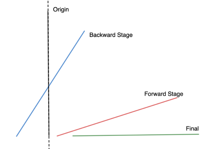
Figure 1. A ruler stands on the table and then sets free with a small angle between the vertical direction, the ruler starts to topple with a horizontal displacement.

One crucial conclusion from observation is that this phenomenon is closely related to the coefficients of friction. If you put the ruler on a flat, smooth table and release it, you are likely to see both backward and forward movements. Whereas if you put the ruler on a piece of wet tissue and repeat the experiment, you probably only find forward sliding exists. The contrast between the two experiments leads to our conclusion.

In this work, we will figure out how the coefficients of friction relate to the existence of forward and backward sliding. We mainly complete the computation by classical mechanics with computer simulation. The theoretical methods are abandoned since Lagrangian or Hamilton mechanics are not suitable for non-holonomic constraints[1] including friction which is the key to this problem.

In some texts, the same question under a frictionless situation was examined, but it turns out that under a frictional environment, the evaluation can be even more sophisticated. In the next section, we will briefly talk about the reason for sliding. And in section 3 we will finish some theoretical analyses and put our primary focus on the stationary stage because of the complexity of handling dynamic motion manually. And the simulations, including both the static stage and dynamic stage, will be presented in Section 4.

2. Reason of sliding

Before we start theoretical analysis, we explain the reason for sliding. The essential cause of sliding is the friction force from the table is not sufficient to support the horizontal acceleration of the mass center when toppling, so the rod itself has to obtain a horizontal acceleration and apply the inertia force to play the role of supporting the acceleration of the mass center.

Another reason is that the rod under our consideration is a rigid body [2], which is also regarded as an assumption. It is because the rod is a rigid object, so it cannot support acceleration with elastic force by deforming.

The reason why two motion stages exist is due to the variation in the direction of acceleration of the mass center. Imagine the trajectory of the mass center as a quarter circle, and it can be expressed by a combination of trigonometric functions. The expression should also include the coefficient of friction according to the conclusion in Section 1. This combination with properties of trigonometric functions will cause the variation of direction (sign) of acceleration, and lead to two different stages. But the conditions for changing signs will depend on other factors (i.e., \( {μ_{s}},{θ_{0}} \) ) which we will evaluate comprehensively in the next section.

3. Theoretical analysis

We pick the contacting point between the rod and the horizontal surface as the reference point for our computing of physical quantity, therefore the torque caused by friction and normal force can be ignored.

3.1. Stationary stage

We first start with stationary. For this section, we will examine various static friction coefficients \( {μ_{s}} \) and figure out the conditions on \( {μ_{s}} \) for a dynamics sliding stage to exist. In hindsight, most of the equation will depend on \( g/l \) , so we extract it out and compose a dimensionless variable \( T \) as an independent variable for convenience for further analysis.

\( T=t\sqrt[]{\frac{g}{l}}\ \ \ \ \ \ (1) \)

In which, \( t \) is the ordinary time, we regard \( T \) as a reference time.

We presumed the rod is a rigid object, then the moment of inertia of the rod [3] is

\( I=\frac{1}{3}m{l^{2}}\ \ \ \ \ \ (2) \)

With regard to the torques, we have the relationship [4].

\( \frac{{d^{2}}θ}{d{T^{2}}}=\frac{M}{I}=\frac{3}{2}sin{θ}\ \ \ \ \ \ (3) \)

We now apply an initial condition \( θ(0)={θ_{0}},\dot{θ}(0)=0 \) , and the solution of this differentiation equation can be expressed in Jacobian ellipse functions [5]

\( θ(T)=2arcsin\lbrace sin(\frac{{θ_{0}}}{2})cd(i\sqrt[]{\frac{3}{2}}T,{sin^{2}}{(\frac{{θ_{0}}}{2})} )\rbrace \ \ \ \ \ \ (4) \)

For the forces in the horizontal and vertical direction, we suppose the coordinates of the mass center as \( ({x_{C}}, {y_{C}}) \) , and obviously, we can express the magnitude of coordinates as follows

\( {x_{C}}=\frac{l}{2}sin{θ},   {y_{C}}=\frac{l}{2}cos{θ}\ \ \ \ \ \ (5) \)

Where the \( θ \) is the angle between the rod and the vertical. And the second derivative of \( {x_{C}} \) and \( {y_{C}} \) is

\( {\ddot{x}_{c}}=\frac{l}{2}\frac{{d^{2}}θ}{d{t^{2}}}cos{θ}-\frac{l}{2}{(\frac{dθ}{dt})^{2}}sin{θ},   {\ddot{y}_{c}}=-\frac{l}{2}\frac{{d^{2}}θ}{d{t^{2}}}sin{θ}-\frac{l}{2}{(\frac{dθ}{dt})^{2}}cos{θ}\ \ \ \ \ \ (6) \)

Apply Newton's second law in both horizontal and vertical directions

\( \begin{cases} \begin{array}{c} m\cdot {\ddot{y}_{c}}=N-mg \\ m\cdot {\ddot{x}_{c}}={μ_{s}}N \end{array} \end{cases}\ \ \ \ \ \ (7) \)

Note that the less or equal symbol on the second equation, as long as the condition is not satisfied, the stationary state converts to the dynamic state. We present all the constraints in one equation and apply our dimensionless variable T.

\( \frac{{d^{2}}θ}{d{T^{2}}}(\frac{1}{{μ_{s}}}+tan{θ})+{(\frac{dθ}{dT})^{2}}(1-\frac{tan{θ}}{{μ_{s}}})-\frac{2}{cos{θ}}≤0\ \ \ \ \ \ (8) \)

Using energy conservation to find the explicit form of the square of the first derivative of \( θ \)

\( {(\frac{dθ}{dT})^{2}}=3(cos{{θ_{0}}}-cos{θ})\ \ \ \ \ \ (9) \)

Combine with the very first differentiation equation \( \frac{{d^{2}}θ}{d{T^{2}}}=\frac{3}{2}sin{θ} \) , the inequality can be further simplified as follows

\( \frac{3}{2}sin{θ}(\frac{1}{{μ_{s}}}+tan{θ})+3(cos{{θ_{0}}}-cos{θ})(1-\frac{tan{θ}}{{μ_{s}}})≤\frac{2}{cos{θ}}\ \ \ \ \ \ (10) \)

As shown above, the inequality only has three independent variables \( { μ_{s}} \) , \( {θ_{0}}, \) and T. We now want to see for what interval of \( { μ_{s}} \) the dynamic stage is able to occur at some T, i.e. the condition \( m\cdot {ẍ_{C}}≤{μ_{s}}N \) is not satisfied for at least one T value. Trying to solve this equation by brute force is unrealistic, What we can do is evaluate the behavior near limits \( T→0 \) and \( {μ_{s}}→±∞ \) and see how conditions can be satisfied.

We first start with the situation with \( T→0 \) , at the same time \( θ→{θ_{0}} \) . The \( {μ_{s}} \) can be arbitrarily small as long as \( {μ_{s}} \) is greater than zero. So the very first restriction is

\( {μ_{s}}≥0\ \ \ \ \ \ (11) \)

And another task is dealing with the situation in which \( { μ_{s}}→∞ \) . We first resort to our inequality (10) as the following order

\( (\frac{3}{2}sin{θ}-\frac{3}{{μ_{s}}}(cos{{θ_{0}}}-cos{θ}))sin{θ}+(\frac{3}{2{μ_{s}}}sin{θ}+3(cos{{θ_{0}}}-cos{θ}))cos{θ}-2≤0\ \ \ \ \ \ (12) \)

When \( { μ_{s}}→∞ \) , terms which are proportional to \( μ_{s}^{-1} \) are negligible. The inequality becomes

\( \frac{3}{2}{sin^{2}}{θ}+3(cos{{θ_{0}}}-cos{θ})cos{θ}-2≤0\ \ \ \ \ \ (13) \)

Use simple trigonometric identities and simplify, we have

\( -cos{2θ}+4(cos{{θ_{0}}}-cos{θ})cos{θ}≤\frac{5}{3}\ \ \ \ \ \ (14) \)

We evaluate the maximum value of the left-hand side for the above inequality. If the maximum value is greater than 5/3, the rod can still move. And the maximum value occurs at

\( {θ_{max}}=arccos{(\frac{cos{{θ_{0}}}}{3})} Maximum Value \frac{4+cos{2{θ_{0}}}}{3}\ \ \ \ \ \ (15) \)

For limit \( {θ_{0}}=0 \) , maximum value is 5/3. This result is out of expectations, which means that even if static friction is tremendous, the rod still has an instant to start sliding (for a suitable \( {θ_{0}} \) ). The underlying explanation to this is that the normal force has a minimum value depends on the initial angle of the rod (for \( {θ_{0}}→0 \) , the minimum is 0), with some suitable \( { μ_{s}} \) , the driving force is able to overcome static friction since normal force is relatively small. But an alert is that we made a sloppy decision on the sign of the very first inequalities. The exact form should be

\( \begin{cases} \begin{array}{c} m\cdot {\ddot{y}_{c}}=N-mg \\ m\cdot |{\ddot{x}_{c}}|={μ_{s}}N \end{array} \end{cases}\ \ \ \ \ \ (16) \)

Suppose \( {θ_{0}}→0 \) , maximum value occurs at \( arccos{1/3} \) , we need to check the direction of \( {\ddot{x}_{c}} \)

\( {\ddot{x}_{c}}=\frac{3}{4}sin{(arccos{\frac{1}{3}})}×\frac{1}{3}-\frac{3}{2}(1-\frac{1}{3})sin{(arccos{\frac{1}{3}})}=-\frac{\sqrt[]{2}}{2}\ \ \ \ \ \ (17) \)

as shown above, the computed acceleration is in a negative direction, or in other words, the friction should be in a negative direction too ( \( F=ma \) ), and the direction of sliding is opposite to the direction of friction, which is the positive direction. Drop a hint that the rod may have a forward stage without going backward. The experiment we mentioned in Section 1 supports this: If you stand a ruler above a wet tissue, where the friction is relatively larger, and give it a small initial angle, then release it, the ruler first rotates, and moves forward without going backward.

However, if the initial angle is large too, the rod may not be able to overcome the static friction force (i.e. cannot exceed 5/3) and simply stay at the origin. Unfortunately, the exact relationship of it cannot be solved with any manual methods and stated in analytical expressions. In conclusion, for some large \( {μ_{s}} \) , and an indeterminate range of \( {θ_{0}} \) , the rod can still slide, but only in the forward direction. We now put our focus on the premise needed on \( {μ_{s}} \) for the rod to have a backward sliding. We state Equation (9) here again. We state the inequality again here.

\( \frac{3}{2}sin{θ}(\frac{1}{{μ_{s}}}+tan{θ})+3(cos{{θ_{0}}}-cos{θ})(1-\frac{tan{θ}}{{μ_{s}}})≤\frac{2}{cos{θ}}\ \ \ \ \ \ (18) \)

To make the LHS greater than RHS with a maximum \( {μ_{s}} \) , we try to do some qualitative analysis. It's easy to prove that

\( 3(cos{{θ_{0}}}-cos{θ}) \lt \frac{3}{2}sin{θ} \lt 1\ \ \ \ \ \ (19) \)

stands for a large range of \( θ \) , which covers our interest range, since if this relationship is no more established, the second term in inequality takes domination, for maximizing the LHS the \( {μ_{s}} \) will have a trend to turn negative, then friction is in the negative direction, corresponds to a forward motion and is what we aim to avoid in this part of analysis. So to make the LHS relatively larger, we maximize the coefficient of the first term, and at the same time maintain the second term not to be extremely negative. In summary

\( \begin{cases} \begin{array}{c} \frac{3}{2}sin{θ}(\frac{1}{{μ_{s}}}+tan{θ})≥\frac{2}{cos{θ}} \\ 1-\frac{tan{θ}}{{μ_{s}}}≥-ξ \end{array} \end{cases}\ \ \ \ \ \ (20) \)

In which, \( ξ \gt 0 \) is an empirical value, we include this factor since when the first term reaches the maximum value, it may exceed \( 2/cos{θ} \) , therefore, the second term is able to be negative, from numerical simulation we find \( ξ=0.52 \) gives good fits. We list two inequalities together.

\( \frac{tan{θ}}{ξ+1}≤{μ_{s}}≤{(\frac{4}{3sin{θ}cos{θ}}-tan{θ})^{-1}}\ \ \ \ \ \ (21) \)

We take the equal sign and solve out the angle and corresponding time, marking them as \( {θ^{*}} \) and \( {T^{*}} \) , which tell us where and when the LHS reaches maximum. \( {θ^{*}} \) can be solved out in explicit, is \( { θ^{*}}=0.642rad \) .

In the analysis above, \( {μ_{s}} \) only works as an intermediate value, trying to find the maximum value by using the inequality above will only give a rough and inaccurate result, a better opportunity is substituting \( {θ^{*}} \) to the original inequality

\( \frac{3}{2}sin{{θ^{*}}}(\frac{1}{{μ_{s}}}+tan{{θ^{*}}})+3(cos{{θ_{0}}}-cos{{θ^{*}}})(1-\frac{tan{{θ^{*}}}}{{μ_{s}}})-\frac{2}{cos{{θ^{*}}}}=0\ \ \ \ \ \ (22) \)

and solve out \( {μ_{s}} \) , represents as \( μ_{s}^{*} \) , which stands for a rather accurate approximation of the maximum coefficient of static friction for the backward stage. Examples as

\( {θ_{0}}=\frac{5}{180}π,   μ_{s}^{*}=0.371(0);    {θ_{0}}=\frac{15}{180}π,   μ_{s}^{*}=0.396(8)\ \ \ \ \ \ (23) \)

and these approximations fit well.

At the very end, we will take a look at what will happen if \( {θ_{0}}≥0.642 \) rad, i.e. the initial angle already exceeds the angle where the maximum value occurs. In this situation, \( {θ^{*}} \) is simply \( {θ_{0}} \) , the rod starts sliding without a stationary stage. Similarly, \( μ_{s}^{*} \) can be solved by substituting. And the equation is

\( \frac{3}{2}sin{{θ_{0}}}(\frac{1}{{μ_{s}}}+tan{{θ_{0}}})-\frac{2}{cos{{θ_{0}}}}=0\ \ \ \ \ \ (24) \)

Which is much more simplified compared to the previous one. The \( {μ_{s}} \) got from the equation above will still guarantee the existence of backward motion, we can now apply Lagrange multiplier method [6] to find the maximum \( {μ_{s}} \) and corresponding \( {θ_{0}} \) for a backward motion. i.e. we what to find:

\( \begin{cases} \begin{array}{c} Maximum f({μ_{s}},{θ_{0}})={μ_{s}} \\ Restriction g({μ_{s}},{θ_{0}})=\frac{3}{2}sin{{θ_{0}}}(\frac{1}{{μ_{s}}}+tan{{θ_{0}}})-\frac{2}{cos{{θ_{0}}}} \end{array} \end{cases}\ \ \ \ \ \ (25) \)

Applying Lagrange multiplier parameter \( λ \) , and equations are

\( \begin{cases} \begin{array}{c} 1-\frac{3λ}{2μ_{s}^{2}}sin{{θ_{0}}=0} \\ \frac{3}{2}sin{{θ_{0}}}(\frac{1}{{μ_{s}}}+tan{{θ_{0}}})-\frac{2}{cos{{θ_{0}}}}=0 \\ -\frac{λ}{2}sec{{θ_{0}}}tan{{θ_{0}}}+\frac{3λ}{2}cos{{θ_{0}}}(\frac{1}{{μ_{s}}}+tan{{θ_{0}}})=0 \end{array} \end{cases}\ \ \ \ \ \ (26) \)

Which can be solved explicitly, our desired result is

\( μ_{s}^{*}=\frac{3}{4};     {θ_{0}}=arctan{2}\ \ \ \ \ \ (27) \)

So in summary, as long as \( {μ_{s}}≤3/4 \) , you can always find a range of \( {θ_{0}} \) for the mass to slide. The only difference is the existence of stationary stage or in specific \( 0 \lt {θ_{0}} \lt 0.642 \) stationary stages exist, and for other \( {θ_{0}} \) it is absent.

To conclude this whole section, we list all potential situations as following

• For \( 0≤{μ_{s}}≤μ_{s}^{*}, 0 \lt {θ_{0}} \lt 0.642 \) , both stationary stage and dynamic stage present

• For \( 0≤{μ_{s}}≤μ_{s}^{*}, 0.642≤{θ_{0}}≤\frac{π}{2} \) , no stationary stage but dynamic stage presents

• For \( {μ_{s}} \gt μ_{s}^{*} \) , indeterminate, may stay stationary or slide directly forward

3.2. Dynamic stage

When the driving force overcomes static friction force, the rod starts to slide. We include an inertia force in order to describe the following motion within an inertial reference frame. In magnitude

\( {F_{inertia}}=-m\frac{{d^{2}}x}{d{t^{2}}}\ \ \ \ \ \ (28) \)

In which the x is the displacement of the contacting point between the rod and table. Again we suppose the coordinates of the mass center are as above. The equations now become

\( \begin{cases} \begin{array}{c} m\cdot {\ddot{y}_{c}}=N-mg \\ m\cdot {\ddot{x}_{c}}=-sgn(\dot{x})\cdot {μ_{d}}N-m\frac{{d^{2}}x}{d{t^{2}}} \\ \frac{{l^{2}}}{3}m\ddot{θ}=-m\frac{{d^{2}}x}{d{t^{2}}}\frac{l}{2}cos{θ}+mg\frac{l}{2}sin{θ} \end{array} \end{cases}\ \ \ \ \ \ (29) \)

With simplification and applying T (here we set T to start from 0, in actual simulation T should starts at \( {T_{slide}} \) ), we obtain the sophisticated result.

\( \frac{2}{3}\frac{{d^{2}}θ}{d{T^{2}}}=[\frac{1}{2}\frac{{d^{2}}θ}{d{T^{2}}}cos{θ}-\frac{1}{2}{(\frac{dθ}{dT})^{2}}sin{θ}+sgn(\dot{x}){μ_{d}}(-\frac{1}{2}\frac{{d^{2}}θ}{d{T^{2}}}sin{θ}-\frac{1}{2}{(\frac{dθ}{dT})^{2}}cos{θ})]cos{θ}\ \ \ \ \ \ (30) \)

\( +(sgn(\dot{x}){μ_{d}}cos{θ}+sin{θ}) \)

And we write the initial conditions(from the end of the stationary stage) as

\( θ(0)=ϕ,   \dot{θ}(0)=α\ \ \ \ \ \ (31) \)

In which the \( sgn \) gives the sign of a value, we include this to ensure the friction is in the opposite direction of velocity. The impediment to solving this differentiation equation caused us to do no further analysis, for this, we can only take numerical simulation. So the analysis of the dynamic stage will be put into Section 4.

4. Simulation

We have finished the theoretical part of this problem, and now we will use math tools to do simulation. The whole simulation will be separated into 4 parts, stationary, backward, forward, and after-colliding phases.

For the whole simulation, we will still use our reference time \( T \) for simplicity. All degrees are in radius, and the length of the rod is normalized to 1. For a realistic situation, we put \( l \) and \( g \) into consideration, and the ordinary time can be computed with \( t=T\sqrt[]{l/g} \) .

4.1. Stationary stage

We will first evaluate the stationary stage, aiming to verify our conclusion in Section 3. We illustrate the result of simulating in contour plot [7]. The plotted function is

\( f({μ_{s}},{θ_{0}},θ)=hardtanh(\frac{\ddot{{x_{C}}}}{{μ_{s}}N})\ \ \ \ \ \ (32) \)

The hardtanh function [8] restricts all values in range \( [-1,1] \) , which is defined as

\( hardtanh(x)=max(-1,min(1,x))\ \ \ \ \ \ (33) \)

The reason why we use fractions is that with fractions we can distinguish the sign of \( {\ddot{x}_{c}} \) more straightforwardly which makes it easier for us to determine the direction of sliding. To be specific, for those areas with a value of -1 (dark blue) the rod will go forward (the backward stage is absent), and for those areas with a value of 1 (light red), a backward stage exists. We start from the situation where \( {μ_{s}} \) is small \( (0 \lt {μ_{s}} \lt 1) \) .

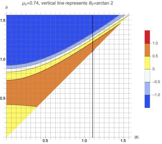
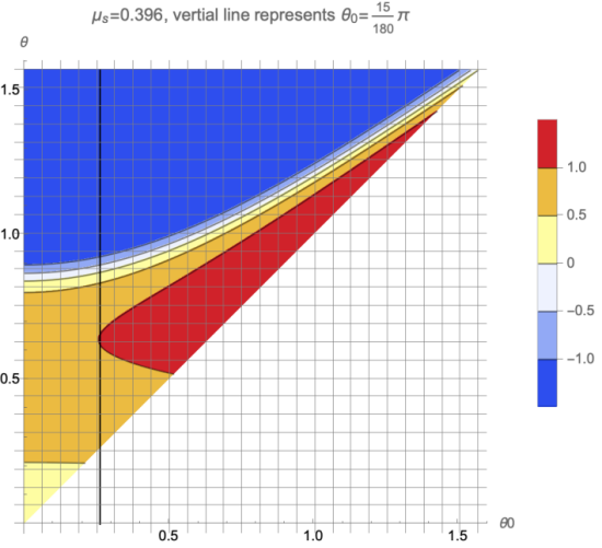
From our analysis in Section 3, \( {μ_{s}}=0.396 \) is the maximum coefficient of static friction for a rod with initial angle \( {θ_{0}}=\frac{15π}{180} \) to make backward motion, and this is proved in the left diagram of Figure 1: If the value of \( {μ_{s}} \) is a bit larger, then the vertical line will lose contact with light red area, i.e., it will present no backward stage. We also predicted that \( {μ_{s}}=0.75 \) is the maximum value for the backward stage to exist. We set \( {μ_{s}}=0.74 \) in the right diagram of Figure 1, which is quite close to 0.75. We can still observe a very small area for light red, which means the rod still has a tiny opportunity to have backward motion. For \( {μ_{s}}=0.75 \) , the last area will completely disappear, with no more backward motion.

And now we start evaluating some large \( {μ_{s}}({μ_{s}} \gt 1) \) . In reality, this kind of friction exists (e.g., Lubricated gold between gold [9]). As shown in Figure 2: For those relatively large \( {μ_{s}} \) , we can still observe a considerable area of value -1, which means the rod will directly go forward after the stationary stage.

Comparing all four diagrams, we conclude that as \( {θ_{0}} \) increases the area of value -1 becomes smaller. As we found in Section 3, even though \( {μ_{s}}→∞ \) , the rod can still slide, and on the diagram, the area with value -1 will become a dot on the \( θ \) axis at \( θ=arccos{(1/3)} \) . However, the relationship between \( {μ_{s}} \) and \( {θ_{0}} \) still can't be expressed in analytical expression.

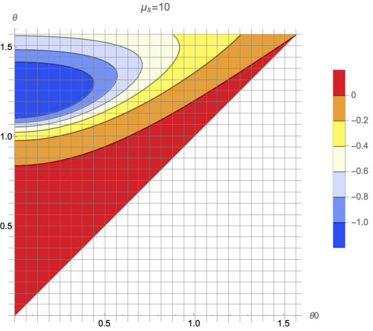
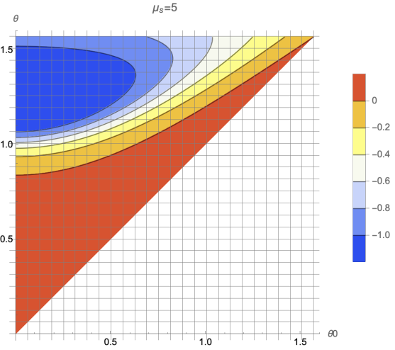
Figure 3. The plot for large \( {μ_{s}} \) . Note that, the light red in the figure no longer represents the area with values equal to 1. In other words, a backward stage has no possibility to exist.

But now with the help of the computer, we can generate the curve that represents the relationship between \( {μ_{s}} \) and \( {θ_{0}} \) . As shown in Figure 3 and Figure 4, which show the relationship for small \( {μ_{s}} \) and large \( {μ_{s}} \) correspondingly.

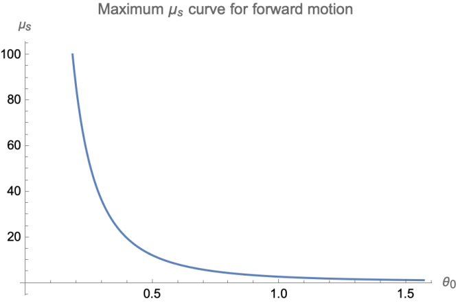
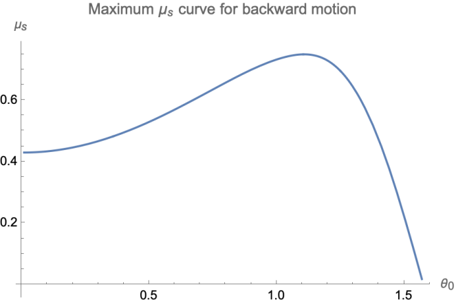
For Figure 3, the maximum point occurs at \( {θ_{0}}=arccos{2} \) and \( {μ_{s}}=0.75 \) . And this is the maximum coefficient of static friction for backward motion as we concluded in Section 3. For Figure 4, the line should contact the \( {θ_{0}} \) axis when \( {θ_{0}}→π/2 \) but because of the scale of the diagram it did not present clearly on the graph. The curve has an asymptote for \( {θ_{0}}→0 \) , at there, the maximum \( {μ_{s}}→∞ \) , comes up with our conclusion in Section 3.

4.2. Dynamic stage

Now we will simulate the dynamic stage. To investigate both backward and forward stages, including the conversion between them, we will take some relatively friendly \( {μ_{s}} \) and \( {θ_{0}} \) and put focus on the effect of varying \( {μ_{d}} \) on the whole dynamic motion.

The main idea of simulating is solving differential equations with the computer, there will be three equations in total: backward sliding, forward sliding, and after colliding with the ground. The first two equations are given in Section 3.2, and the third equation is Newton's second law with a deceleration of \( -{μ_{d}} \) .

As shown in Figure 5, we showed the situation with fixed \( {μ_{s}}=0.3 \) and \( {θ_{0}}=5π/180 \) and different \( {μ_{d}} \) , where according to reality, most of \( {μ_{d}} \) should satisfy restriction \( {μ_{d}}≤{μ_{s}} \) [10]. No matter what value of \( {μ_{d}} \) the forward motion always takes domination, and the value of \( {μ_{d}} \) will only affect the distance of both backward and forward motion.

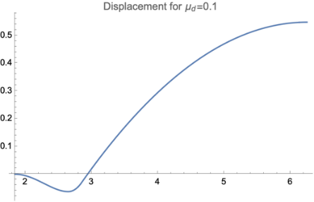
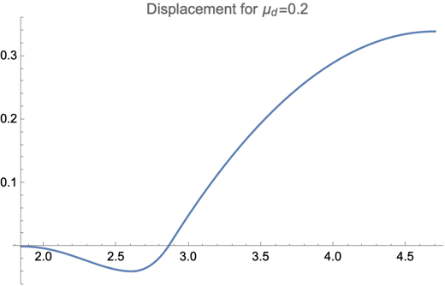
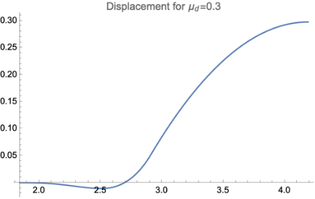
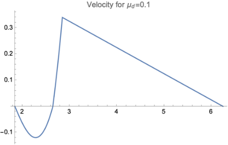
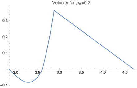
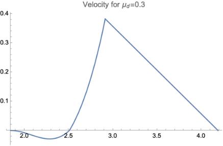
A crucial problem with the graphics is that there exist several turning points which have no physical meaning. The reason why this is present is we used an idealized model of friction, where the conversion from static friction to dynamic friction is a discontinuous jump. If we put a realistic model into use will increase the complexity of the question, which is not the topic of this paper.

And it turns out that, for certain small \( {μ_{s}} \) , the backward sliding will take domination and the rod will stop behind the initial position. For a limit with \( {μ_{s}}=0 \) , the rod experiences no horizontal force, therefore the position of the mass center will not move and the overall effect is a backward sliding with distance l/2.

For \( {θ_{0}}=5π/180 \) the maximum coefficient of static friction for a backward stage to exist is \( {μ_{s}}=0.371 \) and was proved to be true in the last section. And now we will set \( {μ_{s}} \) to 0.4, to investigate the forward motion without a backward stage.

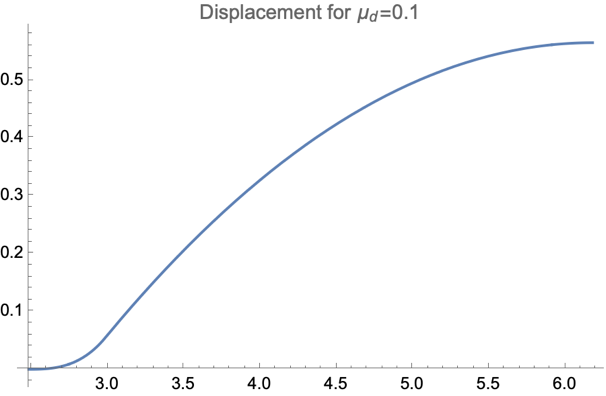
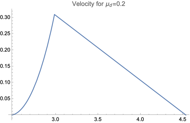
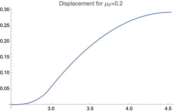
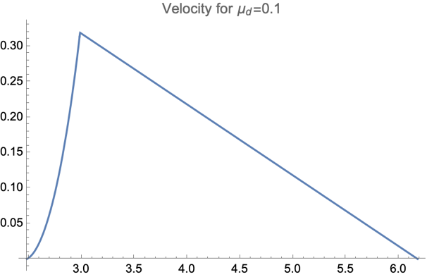
Figure 6. The diagrams for only forward motion. All figures are generated under the situation of \( {μ_{s}}=0.4 \) and \( {θ_{0}}=\frac{5π}{180} \) .

As shown in Figure 6. From the graphics, we can conclude that most of the forward motions occur after the rod collides with the ground, and the moving during toppling only devotes a small amount of distance. The reason for this kind of situation is that the rod starts sliding near the end of rotation( \( θ=0.9rad \) ). Similarly, the variation of \( {μ_{d}} \) will only affect the distance traveled.

5. Conclusion

In this paper, we did a deep investigation into the phenomenon of a toppling ruler. We explained the essential reason for sliding and demonstrated the internal mechanism with theoretical analysis. Finally, we verified our theory with numerical simulation.

The question was found in our daily life, it seems quite obvious and is supposed to be in our common sense, but the exact mechanism and conditions behind it are far beyond our expectations. However, it is also because of its complexity, that the problem was able to have tons of variations and was fun for analyzing.

References

[1]. Louis N Hand and Janet D Finch. Analytical Mechanics. en. Cambridge, England: Cambridge University Press, Nov. 1998.
[2]. Andy Ruina and Rudra Pratap. Introduction to Statics and Dynamics. Oxford University Press, 2015.
[3]. Raymond Serway. Physics for Scientists and Engineers : With modern physics. 2nd ed. Saunders College Publishing, 1986.
[4]. John R Taylor. Classical Mechanics. en. Sausalito, CA: University Science Books, Sept. 2004.
[5]. Carl Gustav Jacob Jacobi. Cambridge Library Collection - Mathematics: Fundamenta nova theoriae functionum ellipticarum. la. Cambridge, England: Cambridge University Press, Nov. 2012.
[6]. Angel de la Fuente. Mathematical methods and models for economists. Cambridge, England: Cambridge University Press, Jan. 2000.
[7]. Wolfram Research, ContourPlot, Wolfram. 1988 https://reference.wolfram.com/language/ref/ ContourPlot.html
[8]. PyTorch Contributors, Hardtanh. 2023 https://pytorch.org/docs/stable/generated/torch.nn. Hardtanh.html
[9]. Mechanical Engineering Department: Tribology Introduction. 2016 http://mechanicalemax. blogspot.com/2016/03/tribology-introduction.html
[10]. Friction Factors – Coefficients of Friction. 2015 https://www.roymech.co.uk/Useful_Tables/ Tribology/co_of_frict.htm
Cite this article
Guo,H. (2023). Research on the bidirectional sliding phenomena of a toppling rod under frictional situations. Theoretical and Natural Science,12,78-87.
Data availability
The datasets used and/or analyzed during the current study will be available from the authors upon reasonable request.
Disclaimer/Publisher's Note
The statements, opinions and data contained in all publications are solely those of the individual author(s) and contributor(s) and not of EWA Publishing and/or the editor(s). EWA Publishing and/or the editor(s) disclaim responsibility for any injury to people or property resulting from any ideas, methods, instructions or products referred to in the content.
About volume
Volume title: Proceedings of the 2023 International Conference on Mathematical Physics and Computational Simulation
© 2024 by the author(s). Licensee EWA Publishing, Oxford, UK. This article is an open access article distributed under the terms and
conditions of the Creative Commons Attribution (CC BY) license. Authors who
publish this series agree to the following terms:
1. Authors retain copyright and grant the series right of first publication with the work simultaneously licensed under a Creative Commons
Attribution License that allows others to share the work with an acknowledgment of the work's authorship and initial publication in this
series.
2. Authors are able to enter into separate, additional contractual arrangements for the non-exclusive distribution of the series's published
version of the work (e.g., post it to an institutional repository or publish it in a book), with an acknowledgment of its initial
publication in this series.
3. Authors are permitted and encouraged to post their work online (e.g., in institutional repositories or on their website) prior to and
during the submission process, as it can lead to productive exchanges, as well as earlier and greater citation of published work (See
Open access policy for details).