1. Introduction

Neural Network is a subset of machine learning technology developed in 20th century. The neuron system of human brain inspired its basic principle design to achieve the function of adjusting the relation parameters between inputs and outputs. Nowadays, the applications of traditional Neural Network can be witnessed in all aspects, including research areas and our daily life technology, like the identification of visual images, voices, and some predictions and analysis in financial and medical areas. The algorithm is modelled based on the dendritic structure of the brain, where the neurons are interconnected and able to receive, process, and transmit data. The basic principle is that each neuron receives the sum of the multiplications of inputs and their corresponding weights. After processing by a nonlinear function, an output is generated, and passed down to the neurons of the next layer and so on. These layers of neurons create a system carrying the nonlinear correlations of high complexity data showing much stronger power than basic linear regression methods [1].

In supervised learning, to find the accurate weights mentioned above to fix the correlation, the Neural Network uses ‘back propagation’ to adapt the weights and bias. The principle of ‘back propagation’ is using given training datasets, calculating the cost function for each neuron, and iteratively adjusting the weights to lower the cost functions and reach the best pattern. For the case of unsupervised learning, it is more complicated as there is no training set, and the classification process depends completely on the features of the data [1]. Nevertheless, the traditional Neural Network has already shown its limitations when extending its application. For example, it is vulnerable to over-fitting, which means the Neural Network is too specialized to the training set that it performs poorly in the training set. In addition, the traditional Neural Network demands a considerable number of computational resources in training and running processes. The low efficiency limits the algorithm’s applications in many aspects.

However, in the 21st century, the introduction of the quantum computing field has started a new topic called ‘Quantum Neural Networks (QNN)’. In the context of quantum computing, the Quantum Neural Network can break through plenty of limitations used to exist in traditional computing, mainly limitations involving its computational power [2]. While classical computers process information using binary bits (0 or 1), quantum computers apply qubits as their foundation by preparing quantum particles. A particle representing a qubit can exist in either 0 or 1 with specific probabilities. This superposition property gives vital advantages over traditional computing, e.g., quantum parallelism and quantum entanglement, so that quantum computers can store and process exponentially more information than traditional computers do [3].

Making full use of the characteristics of quantum computing, QNN can realize a much more enhanced processing power; the quantum entanglement property can lead to new intrinsic links between neurons. Besides, QNN will have a very high potential for new algorithms to be explored. Here are some essential researches during its development. In 2019, Havlíček and his team proposed a quantum kernel-based method to realize some classical supervised learning tasks, showing the possibility of combining quantum computing and neural network [4]. In 2018, Farhi and Neven introduced a QNN that was applicable to some near-term quantum processors. By comparing its accuracy with the outcomes of the classical Neural Network, the paper showed the QNN’s feasibility and potential [5]. In 2020, Beer and his team proposes and designs a quantum neural network that performs tasks similarly to classical neurons. The quantum feedforward neural networks can be applied in universal quantum computation [6]. The motivation of this review paper is to conclude and study the latest research process on QNN so far, its applications, and future development. In the following content of the paper, the article consists of five sections, the principle of QNN, the algorithms, the applications, the limitations and future outlooks, and the conclusion.

2. Principle

As the computing unit of the computing is transferred from bits to qubits, the basic principle of the algorithms is completely altered. |·> and <·| are called Dirac notations which are commonly used in quantum computing, introduced by Paul Dirac. They are also called bracket notations, which are column vectors and row vectors, respectively; <x|y> denotes the inner product, which gives out a scalar quantity. |x><y| denotes the outer product, which represents a matrix operator. Here, |x> stands for a linear combination of the basis states. In quantum computing, the basis set is {|0>, |1>}:

|x> = a|0> + b|1> (1)

The parameters are complex and should be normalized:

|a|² + |b|² = 1(2)

Therefore, a qubit can be represented by a two-times-one column vector. a and b carry the information of the probabilities of the state of the qubit after collapsing (one of the basis states), so they are also called probability amplitude, and the probabilities are |a|² and |b|². In addition, qubits can be represented using real parameters:

|x>= e^iy cosΦ|0>+ e^iδsinΦ|1>(3)

where y, δ, Φ are real quantities [2].

3. Properties

After introducing the basic logic of quantum computing, there are some intrinsic unique properties that make quantum computing in some way superior to classical computing that should be fully explored. Quantum entanglement is a phenomenon that occurs in multi-qubit occasions. When there are multiple particles in a system, there are cases where instead of regarding the system as a linear combination of multiple particles, the particles interact and entangle, leading to counterintuitive outcomes [2]. In Dirac notation, one considers two quantum states |x>₁ and |x>₂. |x>₁₂ is the combination of the two states. If |x>₁₂ cannot be expressed as the tensor product of two individual vectors, the state is an entangled state [2]. As in quantum mechanics, particles are expressed in wave form. Interference is a common phenomenon and should be considered in a microcosmic view. Interference happens when two coherent waves are combined constructively or destructively depending on their phase difference [2]. As a qubit has the superposition property mentioned before, instead of carrying one 0-1 information, one qubit can simultaneously exit in both 0 and 1 states. This fundamental logical difference gives quantum computing an exponential advantage over traditional computing, as in theory, quantum computers can conduct multiple calculations in parallel at the same time [3]. For example, suppose a problem needs the computer to try all possible outcomes of the inputs. Instead of sequentially try the inputs one by one, a quantum computer can explore all possibilities simultaneously. However, as the outcome of quantum computing will finally collapse to a particular result, additional measurements are required to extract information from the superposition. Therefore, the advantage of quantum parallelism only exists in some algorithms. It is a great challenge to explore algorithms that can fully realize the theoretical edges lying in quantum parallelism and interference to solve specific problems efficiently [2].

4. Quantum gate

A quantum gate is a component of a quantum computing circuit that has the ability to unitarily transform quantum state vectors. There are single-qubit or two-qubit gate and so on, depending on the number of qubits involved. One of the most basic gates is the single-qubit rotational gate, which performs basic rotation on one qubit’s phase. It can be represented as:

R(Θ) = \( [\begin{matrix}cosΘ & -sinΘ \\ sinΘ & cosΘ \\ \end{matrix}] \) (4)

For a quantum state |Φ>= \( [\begin{matrix}cosΦ \\ sinΦ \\ \end{matrix}] \) :

R(Θ) |Φ> = \( [\begin{matrix}cos(Φ+Θ) \\ sin(Φ+Θ) \\ \end{matrix}] \) (5)

Another essential kind of gates is the Pauli gates. They perform the same function as Pauli matrixes (X, Y, Z). One notable but commonly used gate should be emphasized, the Hadamard gate. Hadamard gate is a single qubit gate, and the unitary matrix representation is shown a

H = \( \frac{1}{\sqrt[]{2}}[\begin{matrix}1 & 1 \\ 1 & -1 \\ \end{matrix}] \) (6)

The function of the gate is that it can turn a certain state of 0 or 1 into uncertain states:

H |0>=1/ \( \sqrt[]{2} \) (|0>+ |1>) (7)

H |1>=1/ \( \sqrt[]{2} \) (|0> - |1>) (8)

There are also a lot of multiple qubit gates like Controlled-NOT gates, Swap gates, and controlled-U gates. CNOT gate (Controlled-NOT gate), as a typical example, can be represented as:

CNOT = \( [\begin{matrix}\begin{matrix}1 & 0 \\ 0 & 1 \\ \end{matrix} & \begin{matrix}0 & 0 \\ 0 & 0 \\ \end{matrix} \\ \begin{matrix}0 & 0 \\ 0 & 0 \\ \end{matrix} & \begin{matrix}0 & 1 \\ 1 & 0 \\ \end{matrix} \\ \end{matrix}] \) (9)

If the first qubit is in state 1, the second qubit will be complemented. Otherwise, the second qubit will remain the same. All kinds of quantum gates and qubits compose the significant compositions of a complete quantum circuit. All algorithms are developed and realized through these essential elements from the ground, so are Quantum Neural Networks [2].

5. QNN models

Till now, many algorithms have been developed for QNN of different principles. The following section will pick and introduce several typical and essential models.

5.1. Quantum M-P neural network

Zhou and Ding proposed the quantum M-P neural network in 2007 [7], which is a preliminary practice of transferring the classical M-P neural network to a quantum neural network. The algorithm’s basic principle and weight updating methods for both orthogonal and non-orthogonal bases are discussed in detail. In a classical M-P neural network, the activation of a neuron is the sum of the inputs (y) multiplied by weights (w). A threshold Θ is set to compare with the sum and decide whether to activate the neuron. If the neuron is activated, the sum will go through a nonlinear function (f), generate the output and pass on to the next layer [7]. To describe the process mathematically:

\( {y_{k}}={Σ_{j}}{a_{j}}{ω_{j}} \) (10)

\( {O_{k}}=f({y_{k}}-θ) \) (11)

where y_k is the input, and O_k is the output of a neuron. To transfer the algorithm from classical computing to quantum computing context, the values should be replaced by the superposition of quantum states. The output is expressed as:

\( {O_{k}}={Σ_{j}}{ω_{kj}}{ϕ_{j}}, j=1,2,…,{2^{n}} \) (12)

Here, Φ stands for the quantum state. n is the number of qubits. If the states are orthogonal to each other:

\( {O_{k}}={Σ_{j}}{ω_{kj}}|{a_{1}},{a_{2}},…,{a_{n}} \gt , j=1,2,…,{2^{n}} \) (13)

where a is the input qubit. To determine the weights of the neural network, the algorithm first initializes a weight matrix. Prepare a training-sample set with input qubits and expected outputs. Calculate the outputs with the inputs through the weight matrix. Update the weights with the formula:

\( ω_{kj}^{c+1}=ω_{kj}^{c}+τ(|o{ \gt _{k}}-|{γ \gt _{k}})|ϕ{ \gt _{j}} \) (14)

where k and j are the row and column numbers, and τ is the learning rate. Do the processes iteratively until the error is small enough [7]. However, the Quantum M-P Neural Network proved to be primitive and problematic. In 2015, Silva et al. showed that this model did not follow the unitary evolution, and the algorithm showed no advantage over the classical algorithms by a simple two-qubit example [8].

5.2. Quantum Hopfield network

In 2018, Patrick and his team proposed the Quantum Hopfield Network, a transfer from the classical Hopfield Network into quantum computing [9]. The model creates an associate memory network in the context of quantum computing. The Hopfield network is an unsupervised-learning neural network consists of one layer as shown in Fig. 1. The updating method adopts an algorithm called the Hebbian learning rule. The basic principle of the rule is that the link between a presynaptic neuron and a postsynaptic neuron is more vital when the occasions that they simultaneously fires are more frequent [9]. If there is a training set of M patterns, the weighting matrix is given as:

\( W=[Σ_{m=1}^{M}{x^{m}}{{x^{m}}^{T}}]/Md -I{I_{d}}/d \) (15)

where m = 1, 2, 3, ...... , M. In a Quantum Neural Network, the classical expression need to be encoded into a Quantum Nural Network expression. In Quantum Hopfield Network, a quantum state needs to be prepared. Furthermore, this can be achieved either through quantum random access memory (qRAM) or efficient quantum state preparation. In this context, Quantum Hebbian learning is developed through classical-to-quantum read-in and the unitary operations performed on the state [9].

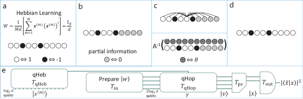
Figure 1. The classical and quantum Hopfield networks [9]. (a) The training process of classical and matrix inversion approaches. (b) The read-in process of classical and matrix inversion approaches. (c) The operation process of classical and matrix inversion approaches. (d) The read-out process of classical and matrix inversion approaches. (e) The whole process of quantum approach.

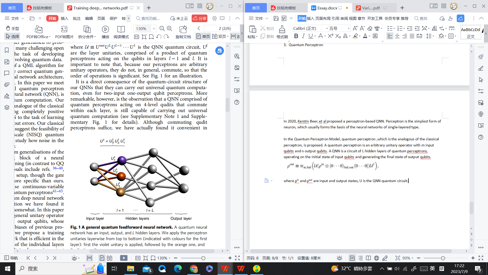
Figure 2. A general quantum feedforward neural network [6].

5.3. Quantum perceptron

In 2020, Kerstin Beer et al. proposed a perceptron-based QNN [6]. Perceptron is the simplest form of neuron, which usually forms the basis of the neural networks of single-layered type (as sketched in Fig. 2). The model is constructed with a quantum perceptron as its analogous classical perceptron. A quantum perceptron has certain numbers of inputs and outputs and exists in the form of a unitary matrix operator. A QNN is a circuit of several hidden quantum perceptron layers, rotating the initial state of input qubits and generating the final state of output qubits. This QNN can conduct universal quantum computation, and it is also observed that a QNN of 4-level qubits, which commute within their layers, can still conduct universal quantum computation [6].

There are two ways of classical-to-quantum encoding. One is that the distribution is transferred into the distribution of the probabilities of the quantum states. The other is that each sample corresponds to one quantum state. Usually, the training set needs repeatable access [6]. The edge of this model over the classical prototype is evident as the number of qubits compared to bits is decreased exponentially. After trying the model on unknown unitary, the model proved to have great robustness to noise in the training set [6].

5.4. Quantum convolutional neural networks

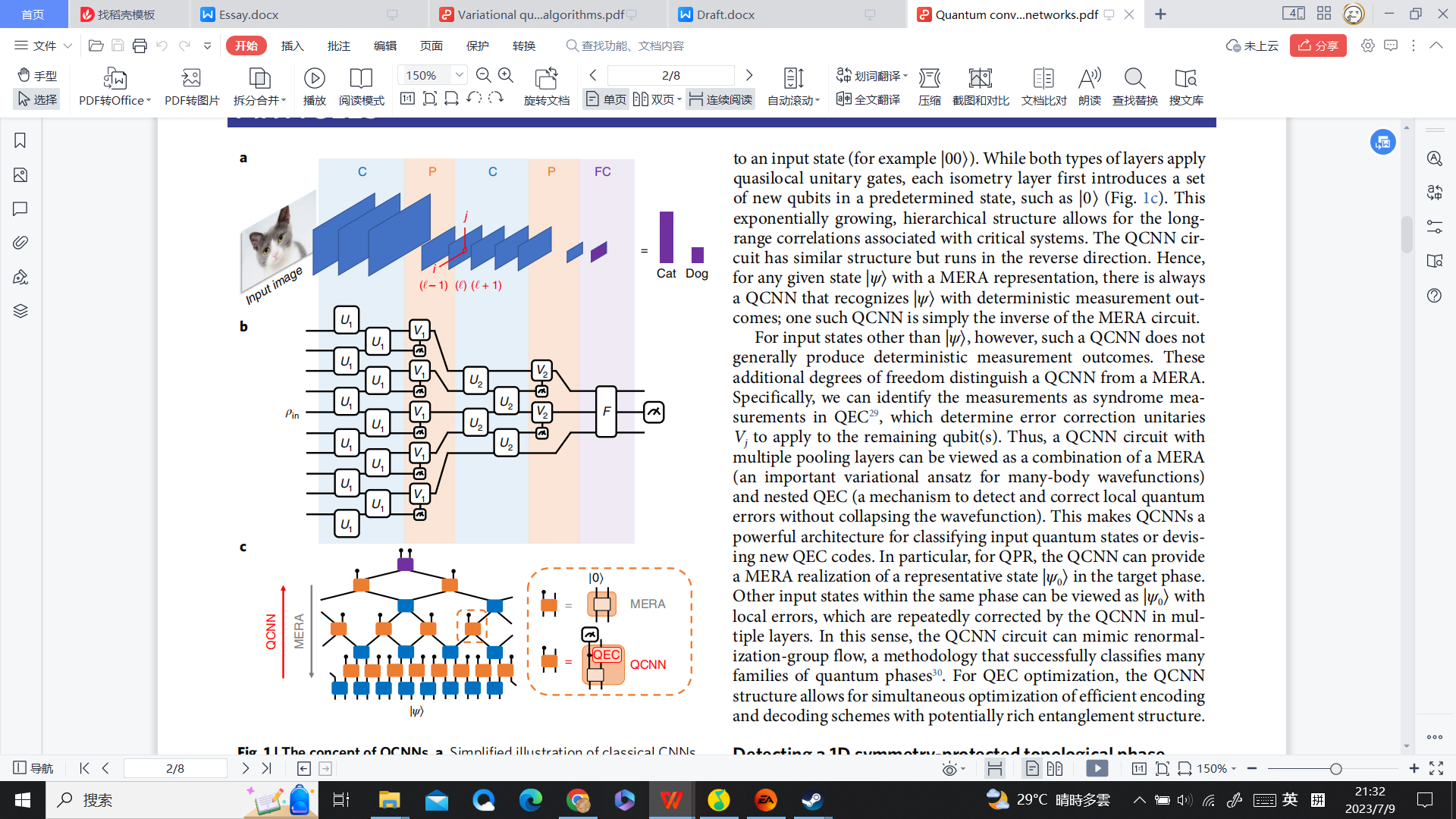
Quantum Convolutional Neural Networks (QCNN), a quantum version of convolutional neural network, were introduced in 2019 by Iris Cong et al. [10]. The Convolutional Neural Network is a neural network designed for processing grid-like data, typically like image and many-body physics problems. The network consists of convolutional layers, pooling layers, and fully connected layers. The filter layers convolve through the whole grid to extract the local feature information from the data. The pooling layers select over the map extracted through the convolutional layers to filter out useless data information. The fully connected layers are similar to the traditional neural networks, which are layers of fully connected neurons, to realize the classifications and the extractions of features [10]. A sketch is illustrated in Fig. 3. The QCNN leverages the computing power of quantum computing into CNN. The grid-like data is transferred into a quantum state. The convolutional layers apply a unitary (Ui) on the data, and similarly, the pooling layers and the fully connected layers are translated into unitary rotation of the matrix (V_j and F). F is updated in the learning process like classical networks [10]. CNN has already been very frequently used, especially in image identification. However, one significant problem of the process has always been the computation resources consumed. The QCNN has a great potential of exponentially reducing the calculation consumption, and greatly extending the application [10].

6. Applications

Many works, some have been introduced before, have been done to realize the transfer from classical machine learning algorithms to quantum computing algorithms and have shown promising potential. The advantages of quantum parallelism, quantum entangling, and great computing power broaden the application area and potential of traditional machine learning. Some typical applications of QNN are image compression, pattern recognition, classifications of data, curve fitting and temperature control. Some vital researches on the application of QNN are also given. Franken and Georgiev explored several quantum circuits in some basic image recognition in 2020 [11]. Although the problem is fundamental, the QCNN showed its noise reduction ability and computation power edge potential. In Liu et al.’s research in 2020, a quantum Hopfield neural network is designed and used in image recognition [12]. The simulation showed its feasibility. In 2018, Farhi, Edward, and Hartmut designed a practical QNN and trained it with a training set of strings and their binary classifications [5]. The feasibility and potential are proven in the area of classification.

7. Limitations and prospects

The Quantum Computing, including Quantum Neural Networks as its branch field, is still in its early stage of development. More and more models from classical algorithms are transferred to the quantum computing context after some adaption. New exclusive quantum algorithms are also proposed. In the next several years, the unique properties of quantum computing will be further explored to realize the theoretical exponential advantage. However, the development in theoretical areas and algorithms is far beyond the hardware development. As the fragility of quantum computers to noise, every increase in qubit number is a revolutionary progress. Due to quantum computers' physical limitations, the majority of the algorithms’ advantages over classical computing remain at the theoretical level. Moreover, the applications of quantum computing lack competitiveness from the economical and practical perspectives due to the high resource of quantum computers. Hence, the world is looking forward to the development of quantum computer facilities.

8. Conclusion

In summary, this paper has introduced the Quantum Neural Network from the basic principle. The basic properties and advantages of quantum neural networks, including the basic quantum computational logic, are introduced. Then, this paper lists a series of typical QNN models to illustrate the algorithm and briefly introduce some current applications of QNN. Finally, the limitations and future development of QNN are stated to provide a big picture. This paper provides a summary of QNN, but many newly developed QNN algorithms are not included and introduced. The algorithms are also in the progress of rapid development currently. The article can only serve as a brief preliminary overview of the topic. In the future, with the research progress of QNN updated, more algorithms and more powerful and striking applications and experiments are expected. The QNN will benefit all human beings in research development and daily life usage.

References

[1]. Abiodun O I, Jantan A, Omolara A E, Dada K V, Mohamed N A and Arshad H 2018 Heliyon vol 4 p 11.
[2]. Jeswal S K and Chakraverty S 2019 Archives of Computational Methods in Engineering vol 26 pp 793-807.
[3]. Vizzotto J K 2013 In 2013 2nd Workshop-School on Theoretical Computer Science pp. 9-13.
[4]. Havlíček V, Córcoles A D, Temme K, et al. 2019 Nature vol 567(7747) pp 209-212.
[5]. Farhi E, and Neven H 2018 arXiv preprint arXiv:1802.06002.
[6]. Beer K, Bondarenko D, Farrelly T et al. 2020 Nature communications vol 11(1) p 808.
[7]. Zhou R and Ding Q. (2007). International Journal of Theoretical Physics vol 46 pp 3209-3215.
[8]. da Silva A J, de Oliveira W R and Ludermir T B 2015 International Journal of Theoretical Physics vol 54 pp 1878-1881.
[9]. Rebentrost P, Bromley T R, Weedbrook C and Lloyd S 2018 Physical Review A vol 98(4) p 042308.
[10]. Cong I, Choi S and Lukin M D 2019 Nature Physics vol 15(12) pp 1273-1278.
[11]. Franken L, and Georgiev B 2020 ESANN vol 11 pp 297-302.
[12]. Liu G, Ma W P, Cao H and Lyu L D 2020 Laser Physics Letters vol 17(4) p 045201.
Cite this article
Li,B. (2023). Analysis of the principle and state-of-art applications for quantum neural network. Theoretical and Natural Science,12,94-100.
Data availability
The datasets used and/or analyzed during the current study will be available from the authors upon reasonable request.
Disclaimer/Publisher's Note
The statements, opinions and data contained in all publications are solely those of the individual author(s) and contributor(s) and not of EWA Publishing and/or the editor(s). EWA Publishing and/or the editor(s) disclaim responsibility for any injury to people or property resulting from any ideas, methods, instructions or products referred to in the content.
About volume
Volume title: Proceedings of the 2023 International Conference on Mathematical Physics and Computational Simulation
© 2024 by the author(s). Licensee EWA Publishing, Oxford, UK. This article is an open access article distributed under the terms and
conditions of the Creative Commons Attribution (CC BY) license. Authors who
publish this series agree to the following terms:
1. Authors retain copyright and grant the series right of first publication with the work simultaneously licensed under a Creative Commons
Attribution License that allows others to share the work with an acknowledgment of the work's authorship and initial publication in this
series.
2. Authors are able to enter into separate, additional contractual arrangements for the non-exclusive distribution of the series's published
version of the work (e.g., post it to an institutional repository or publish it in a book), with an acknowledgment of its initial
publication in this series.
3. Authors are permitted and encouraged to post their work online (e.g., in institutional repositories or on their website) prior to and
during the submission process, as it can lead to productive exchanges, as well as earlier and greater citation of published work (See
Open access policy for details).