1. Introduction

In the past several decades, researchers have witnessed a methodological renaissance that makes problem-solving of complex tasks possible. Methods like causal inference have been applied at different aspects of educational research. In this article, we will explore the topic of educational effectiveness research, which investigates all academic and social development factors affecting the learning outcomes of students, via causal inference and different regression methods. In particular, we will address (1) causal effect of ECLS program on students’ fifth grade math score and (2) factors heavily impacting students’ fifth grade math score. We begin by reviewing four fundamental causal inference frameworks, machine learning in causal inference and the dataset our study is based on in section two. We then describe the methodology in section three, which are the propensity score matching as causal inference tool and three machine learning algorithms, linear regression (LP), multilayer perceptron (MLP) and Bayesian Additive Regression Trees (BART), as regression tools. We finally present and discuss results in section four.

2. Literature review

In this section, we first overview four fundamental casual inference frameworks. In particular, we describe the major parts of each framework and list some of recent works that base on these frameworks. Then we talk about how traditional machine learning methods are applied in context of causal inference by discussing some typical causal machine learning models. And finally, we give a brief introduction to the dataset that is used in this paper.

2.1. Casual inference

Causality helps scientists understand response of a dependent variable when a cause of the effect variable is changed. There are two main conceptual frameworks to tackle casual inference problems, which are causal diagrams and counterfactual models.

A causal diagram is a directed graph which reflects the causal relationship among variables. The idea is firstly proposed by Judea Pearl, which aims to show how graphical models serve as a mathematical language for interpreting statistical information [1]. A causal diagram includes a bunch of nodes, which represent different variables under consideration, and arrows, which represent potential causal effects of parent nodes on their children node. The direction of arrow indicates the direction of causality. The path is the traversal of casual diagram according to the casual arrow direction. There are mainly two types of causal diagrams – causal loop diagrams and directed acyclic graphs. Each one of them serves for different purposes. The causal loop diagrams are cyclic directed diagrams, which visualize dynamic system’s structure and behavior. Two basic types of causal loops are always examined – reinforcing and balancing. Reinforcing loop indicates the change in one direction accumulates more change in that direction and balancing loop means the opposite – change in one direction triggers change in the opposite direction. By determining the loops are reinforcing or balancing, one could quickly draw conclusion the behavior of the system over time, such as how different variables are interrelated in a dynamic system. Some work [2,3] utilize causal loop strong capability to capture the relationships within a system’s structure to decompose and simplify complex problems. Directed acyclic graphs is complement part to causal loop diagrams, which lacks the cycle in the system. The intuition of using directed acyclic graphs (DAG) to explore causal inference is that, in some case, causality assumes events could only affect the future rather than the past and thus lack the causal loops. Compared with its companion causal loop diagrams, directed acyclic graphs is a simpler version of casualty representation in diagram and is suitable to determine if a given pair of variables are independent. Some work [1, 4] use DAGs as a tool to figure out and address potential source of confounding and selection bias in causal inference.

Causal graphs are convenient for displaying qualitative interrelationship among variables. If precise quantitative deductions are needed, method like potential-outcome model [5], which is sometimes called counterfactual model, is an option. The framework of potential-outcome, which is the foundation of the Rubin Causal Model (RCM) [6], estimates the quantitative results based on whether the individual receives the treatment. A set of potential outcomes that could be observed in alternative states of the world, which are counterfactual, helps deducing the causal effect of that particular treatment. Since causal effects on individuals could not be observed directly, the inferential goal of estimating the treatment effect is at the population level, by taking the average, rather than at the individual unit. Two causal assumptions are required to make RCM work properly, which are strong ignorability and stable unit treatment value assumption (SUTVA). Strong ignorability is mathematically formulated as \( \lbrace Y(0),Y(1)\rbrace ⫫ Z | X \) , where \( Y(i) \) is a potential outcome given treatment t, \( X \) is some covariate and \( Z \) is the actual treatment. This assumption says that the potential outcomes are independent of treatment assignment conditioned on observed covariates \( X \) . The SUTVA, on the other hand, holds when the treatment status of any unit does not affect the potential outcomes of other units and the treatment for all units are comparable. In other word, the SUTVA requires the outcome of a particular unit depends only on the treatment to which the unit was assigned, not the treatments of other units. Some work [7, 8] designed different matching mechanism to make assignment process as independent as possible and thus reduce selection bias. If the two conditions are fulfilled, the expected value of causal effect could be approximated by expected outcome of treatment group minus expected outcome of control group.

In this paper, we utilize the second method mentioned above, potential outcome framework, to search for causal inference. In particular, we use the propensity score matching based RCM to determine to what extent a special program affects a primary students’ math score. The propensity score matching reduces the bias due to confounding variables via constructing an artificial control group by pairing treated and non-treated units according to their covariate similarity. Therefore, the propensity score matching based RCM could accurately estimates the impact of an intervention such as this special program.

2.2. Machine learning in casual inference

Thanks to the availability of big data, machine learning could utilize these data to perform high-performance casual inference. Several methods utilize machine learning method to evaluate average treatment effect. The Causal K-Nearest-Neighborhood (i.e., CKNN) has been proposed to do casual discovery [9]. The CKNN method compares the causal treatment effects within near neighborhood which is calculated by traditional KNN rule. Causal random forest (i.e., CRF) is another way to do casual inference, which is built as an extension of traditional random forest [10]. Instead of repeatedly splitting the data in order to minimize prediction error like tradition random forest, CRF splits the data with the purpose of maximizing the difference across groups in terms of relationship between outcome and treatment variables. Causal support vector machine is also used to explore casual inference by balancing covariates and estimating average treatment effect [11]. The dual coefficients are applied on soft-margin SVM classifier as kernel balancing weights, which are used for stable casual effect estimation. Bayesian additive regression trees (i.e., BART), as a recently proposed regression method, plays a role in ensembled methods due to its advantages of finding treatment-covariate interactions and expressing such interactions in a flexible way [12, 13]. By constrained by regularization priors and inferenced by an iterative Bayesian backfitting MCMC algorithm, this BART-based approach not only explores causal inference in an unstructured way but also avoids the pitfalls of data dredging and multiple comparisons.

We mention these machine learning methods only for providing additional information regarding to cutting-edge approaches for causal inference. In this paper, we will use the traditional RCM method and compare it with a basic machine-learning based method, like linear regression.

2.3. ECLS-K dataset

The Early Childhood Longitudinal Studies, Kindergarten Class of 1998–99 (ECLS-K) data is a dataset recording children’s early school experience from a representative sample of children, which is collected by direct child assessment, parent interview, school administrator questionnaires and students’ record. The ECLS-K has two main advantage: large sample size and authority of dataset. The large sample size gives a better generalized estimated result on the underlying population. The authority of dataset gives more reliability of final result due to formal data collection instrument. Many recent papers base their work on the ECLS-K dataset to explore relationship among dataset’s covariates. One of them utilizes the data existing in current ECLS-K to explore the relative contribution of parenting behaviors to SRL and other student outcomes [14]. Another paper examines potential peer effects of English Language Learner students on their non-ELL classmates based on ECLS-K dataset [15]. Even a study utilizes ECLS-K dataset as evidence to disprove the statement that enrolling children in martial arts improves their mental health [16].

We study the ECLS-K dataset in order to better understand effects of different covariates on students’ math score. By examining these interrelationships among covariates, the researcher could help students who are disadvantages in math score.

3. Method

This section is talking about the different methodologies that are used to analyze the ECLS-K dataset. The general objectives of this study are to (1) estimate average treatment effect of ECLS-K program on primary student’s math score and to (2) identify factors that affect primary student’s math score. In order to achieve the first goal, this study bases on the propensity score matching to estimate the potential outcome difference. In order to accomplish the second goal of finding each factor’s contribution to the final math score, three regression models are used to find the relationship between math score and each of considered factors, which are linear regression (LP), multilayer perceptron (MLP) and Bayesian Additive Regression Trees (BART).

3.1. Causal inference by RCM

The Rubin causal model (RCM) is a non-parametric statistical framework which is widely used in causal inference. The RCM defines potential outcomes in terms of difference between observed and counterfactual variables. Due to unobservability nature of counterfactual variables, RCM approximates average causal effect by all the quantities that could be observed based on the assumption that treatment variable assignment is random and is independent of potential outcome. The approximation is calculated in the following form:

\( ATE(Z→Y)=E\lbrace {Y_{i}}(1)-{Y_{i}}(0)\rbrace =E\lbrace {Y_{i}}|{Z_{i}}=1\rbrace -E\lbrace {Y_{i}}|{Z_{i}}=0\rbrace \ \ \ (1) \)

The ATE is abbreviation of Average Treatment Effect, \( {Z_{i}} \) is binary treatment variable of ith example. \( {Y_{i}} \) is outcome variable of ith example. \( \lbrace {Y_{i}}(1),{Y_{i}}(0)\rbrace \) are potential outcomes of ith example. \( {Y_{i}}(1)-{Y_{i}}(0) \) represents casual effect of ith example. The RCM has been shown that it is useful in estimating causal inference [17]. It has been widely used in different areas. One social study which concludes that the employer supplemental insurance is exogenous to the employees' medical care utilization is based on the RCM framework [18]. Another economical study explores the RCM usage in the context of econometric models [19].

3.2. Regression by LR, MLP and BART

The first model is linear regression, which assumes the relationship between dependent and independent variable is linear. In linear regression, linear models are applied to measure unknown model parameters. A particular form of linear regression depends on the nature of problem. In our problem setting, multiple linear regression is suitable. The general form of multiple linear regression is given by:

\( Y={β_{0}}+ {β_{1}}{x_{1}}+ {β_{2}}{x_{2}}+…+{β_{k}}{x_{k}}+ €\ \ \ (2) \)

\( {β_{0}} \) is the intercept and \( {β_{i}} \) is coefficient of \( {x_{i}} \) . \( Y \) is the response. \( € \) is ith disturbance term. Although linear relationship assumption overlooks complicated joint effect of explanatory variables on final prediction, linear regression works well in many circumstances. Even in some complicated settings like observational astronomy, linear regression is preferred in measurement such as cosmic distance scale [20]. The second model is multi-layer perceptron (MLP), which accounts for the situation that relationship between dependent and independent variable is nonlinear. MLP is a fully connected class of ANN, which consists of at least three types of layer: input layer, hidden layer and output layer. The neuron in hidden and output layer uses a nonlinear activation function. The MLP learns a non-linear function approximator that maps input dimension to output dimension by training input dataset. The training uses a supervised learning technique called backpropagation and mean square error loss function for regression. The MLP’s mathematical formulation is shown below:

\( f(x)={W_{2}}g(W_{1}^{T}X+{b_{1}})+{b_{2}}\ \ \ (3) \)

\( g(z)=max{(0,z)}\ \ \ (4) \)

\( {W_{1 }}{,W_{2}} \) are weights of input and hidden layer, \( x \) is input, \( {b_{1}} \) and \( {b_{2}} \) are bias. The function \( g \) is ReLU activation function. The MLP is a very strong technique, which is able to approximate any continuous function in theory. Some recent work [21, 22, 23] apply MLP in complicated setting such as medical diagnosing system, stock price prediction and various optimization algorithm. The last model is Bayesian Additive Regression Tree (BART), which captures not only single variable’s main effect but also multiple variable’s interaction effect on final prediction. BART consists of two parts – a sum-of-trees model and a regularization prior on the parameters of that model. Like traditional ensemble methods like random forest or gradient boosting machine, BART is a sum-of-trees model that regresses an unknown function. Each subtree in BART is a weaker learner which performs slightly better than random guesses. By combining these weak decision tree, BART becomes a strong learner with high predictive accuracy. With the purpose of alleviating the overfitting problem due to nature of ensemble methods, three additional regularization priors are introduced to in a such way that makes (1) depth of tree shallow, (2) parameter value of each learner’s terminal nodes close to 0 and (3) variance of residual noise small. Given the observed data and priors mentioned above, the Bayesian setup induces the posterior distribution that provides parameter space for backfitting MCMC algorithm [12] to get the point estimate for any test data. The sum-of-trees model part can be explicitly expressed in following mathematical formula:

\( y= \sum _{j=1}^{m}g(x;{T_{j}},{M_{j}})+ ϵ\ \ \ (5) \)

\( y \) is the output. x is the input. \( {T_{j}} \) denotes a binary decision tree. \( {M_{j}} \) denotes a set of parameter values associated with each of terminal nodes in a jth binary tree. Given \( T \) and \( M \) , the function \( g(x,T,M) \) assigns a value according to input that contributes to final prediction. \( ϵ \) is gaussian noise with standard deviation \( σ \) .The regularization prior is expressed as following mathematical formula under independent assumption:

\( p(({T_{1}},{M_{1}}),…,({T_{m}},{M_{m}}),σ)=[\prod _{j}^{m}p({M_{j}}|{T_{j}})p({T_{j}})]p(σ)\ \ \ (6) \)

\( p({M_{j}}|{T_{j}})= \prod _{j}p({μ_{ij}}|{T_{j}})\ \ \ (7) \)

p refers to probability. \( {μ_{ij}} \) is element in corresponding \( {M_{j}} \) . The three priors are \( p({T_{j}}) \) , \( p({μ_{ij}}|{T_{j}}) \) and \( p(σ) \) . The \( p({T_{j}}) \) is specified by three aspects – (1) deep nonterminal nodes are unlikely to exist, (2) the distribution on splitting variable assignment is uniform and (3) the distribution on splitting rule assignment is uniform. The \( p({μ_{ij}}|{T_{j}}) \) applies greater shrinkage to parameter values of every terminal nodes as number of subtrees increases in the model. The \( p(σ) \) is correlated to inverse chi-square distribution of degree of freedom. Because of excellent predictive performance for both continuous and binary outcomes, BART has been applied in many important areas such as survival analysis in medical study [24], species distribution modelling in ecology [25] and phenotypes prediction in genomics [26].

4. Results

In this section, we apply methods mentioned in section 3 to identify (1) average treatment effect of ECLS-K program on students’ fifth grade math score and (2) factors heavily impacting students’ fifth grade math score. The dataset we are using is ECLS-K dataset. The variables of dataset are listed below, where d stands for Standardized Mean Difference and r stands for Variance ratio.

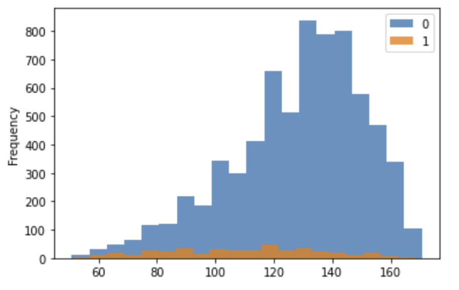
The task of finding ATE is achieved by propensity score matching and linear regression. As been discussed before, the strong ignorability is necessary assumption for RCM to work properly. However, this assumption does not hold for the raw ECLS-K dataset since it is not a randomized trial. Children who receives the treatment are students with learning difficulty. The distribution of control group and treatment groups are shown in histogram below (where 0 represents controlled unit and 1 represents treated unit).

In order to fulfill this assumption, some quasi-experimental methods have to be applied to emulate a randomized study. We resolve to propensity score matching (PSM), which pairs treated and controlled units based on a single-dimension propensity score. We use the trimmed PSM in this experiment, which excludes subjects with extreme propensity score and focuses on those units exhibits high degree of covariates overlapping to make the pairing easy. The results of trimmed PSM are shown below.

According to the table shown above, the estimated average treatment effect is -9.147 with standard error 2.444. The trimmed PSM shows that the ECLS training program has a negative effect on students’ fifth math score.

We also use another machine learning based model, linear regression, as an auxiliary to check the validity of the above trimmed PSM conclusion. Fitting linear model to the data by linear regression, we get formula

\( Y= α+ βX+ γD\ \ \ (8) \)

\( Y \) represents the response which is students’ fifth grade. \( D \) represents the treatment which is the ECLS training program. And \( X \) represents confounding variables which are those remaining variables. Alpha, beta and gamma are coefficients we are trying to solve. After configuring the linear model mentioned above and solving it via ordinary least square, we get the results shown below.

According to the table shown above, the estimated average treatment effect is -7.909 with standard error 0.961. Both the trimmed PSM and linear regression share the similar trend in estimating the average treatment effect of ECLS-K program. Therefore, it is now safe to conclude that the ECLS training program has a negative effect on students’ fifth math score.

The task of finding relationship between math score and each variable is achieved by linear regression, MLP regression and BART. By setting ground truth as students’ fifth grade math score and all other variables as features, linear regression shows that the top three factors that positively impact students’ math score are kindergarten math score, fine motor skill and gender. The top three factors that negatively impact students’ math score are child’s age at k entry, ECLS training program, attended head start. With the purpose of checking the reliability of linear regressor, we split the data into training and test part, where we train the model with training part data and test the trained model with test part data. The root mean squared error (RMSE) of the trained linear model is 15.685, which is not good enough. The second method that we use, the MLP regressor, is set up with 1 hidden layer and ReLU activation for convenience of understanding relationships. The MLP regressor is trained by Adam solver and nesterovs momentum with maximum training iteration 10000. The results of MLP regressor match those of the linear regressor. The three top positive factors are still kindergarten math score, fine motor skill and gender and the three most negative factors are still ECLS training program, child’s age at k entry and attended head start. The RMSE of the MLP model is 16.385, which is a little bit worse than that of linear model. Finally, BART is introduced to improve the model’s performance on unseen dataset. The number of trees is set to 50. The shape and scale parameter of the prior on sigma are both set to 0.001. And the prior parameter on tree structure alpha and beta are set to 0.95 and 2 respectively. The final trained BART model shows the similar relationship trend as linear and MLP model with the lowest RMSE among three methods, which is 15.1.

5. Conclusion

Causal inference plays important roles in educational effectiveness research in that they allow for clarifying complex causal relationship. By above methods, we could conclude that (1) the ECLS-K program has insignificant negative impact on student’s math score, (2) the top three factors that positively impact student’s math score are kindergarten math score, fine motor skill and gender and (3) the top three factors that negatively impact student’s math score are child’s age at k entry, ECLS training program, attended head start. Our results are in accord with those of official analysis, which indicates the receipt of special education services has either a negative or statistically non-significant impact on children’s learning or behaviour [27].

References

[1]. Greenland S, Pearl J, Robins JM. (1999) Causal diagrams for epidemiologic research. Epidemiology. 1999; 10:37–48.
[2]. Bureš,V (2017) A Method for Simplification of Complex Group Causal Loop Diagrams Based on Endogenisation, Encapsulation and Order-Oriented Reduction, 2017
[3]. Brereton, C.F.; Jagals, P.(2021) Applications of Systems Science to Understand and Manage Multiple Influences within Children’s Environmental Health in Least Developed Countries: A Causal Loop Diagram Approach. Int. J. Environ. Res. Public Health 2021, 18, 3010.
[4]. Greenland S, Pearl J. (2014) Causal Diagrams: Wiley StatsRef. Statistics Reference Online; 2014.
[5]. Morgan, S., & Winship, C. (2014). Counterfactuals and Causal Inference: Methods and Principles for Social Research (2nd ed., Analytical Methods for Social Research). Cambridge: Cambridge University Press. doi:10.1017/CBO9781107587991
[6]. Holland, P. W. (1986). Statistics and Causal Inference. Journal of the American Statistical Association, 81(396), 945–960. https://doi.org/10.2307/2289064
[7]. Austin PC. An Introduction to Propensity Score Methods for Reducing the Effects of Confounding in Observational Studies. Multivariate Behav Res. 2011 May;46(3):399-424. doi: 10.1080/00273171.2011.568786. Epub 2011 Jun 8. PMID: 21818162; PMCID: PMC3144483.
[8]. Stuart EA. Matching methods for causal inference: a review and a look forward. Stat Sci 2010; 25:1–21.
[9]. Hitsch, Guenter J. and Misra, Sanjog, Heterogeneous Treatment Effects and Optimal Targeting Policy Evaluation (January 28, 2018). Available at SSRN: https://ssrn.com/abstract=3111957 or http://dx.doi.org/10.2139/ssrn.3111957
[10]. Athey, S., Tibshirani, J., and Wager, S. Generalized random forests. The Annals of Statistics, 47(2): 1148–1178, 2019.
[11]. Ratkovic M. Balancing within the margin: causal effect estimation with support vector machines. Technical report. Princeton, NJ: Department of Politics, Princeton University; 2014.
[12]. Hugh A. Chipman, Edward I. George, Robert E. McCulloch "BART: Bayesian additive regression trees," The Annals of Applied Statistics, Ann. Appl. Stat. 4(1), 266-298, (March 2010)
[13]. Jennifer L. Hill (2011) Bayesian Nonparametric Modeling for Causal Inference, Journal of Computational and Graphical Statistics, 20:1, 217-240, DOI: 10.1198/jcgs.2010.08162
[14]. Min, X., Kushner, S. B., Mudrey-Camino, R., & Steiner, R. (2010). The relationship between parental involvement, self-regulated learning, and reading achievement of fifth graders: A path analysis using the ECLS-K database. Social Psychology of Education, 13(2), 237-269.
[15]. Cho, 2012 R.M. Cho Are there peer effects associated with having English language learner (ELL) classmates? Evidence from the early childhood longitudinal study kindergarten cohort (ECLS-K) Economics of Education Review, 31 (5) (2012), pp. 629 643, 10.1016/j.econedurev.2012.04.006
[16]. Strayhorn, J.M., Strayhorn, J.C. Martial arts as a mental health intervention for children? Evidence from the ECLS-K. Child Adolesc Psychiatry Ment Health 3, 32 (2009). https://doi.org/10.1186/1753-2000-3-32
[17]. Imbens, G.W., Rubin, D.B. (2010). Rubin Causal Model. In: Durlauf, S.N., Blume, L.E. (eds) Microeconometrics. The New Palgrave Economics Collection. Palgrave Macmillan, London. https://doi.org/10.1057/9780230280816_28
[18]. Albouy, Valerie and Crepon, Bruno, Moral Hazard and Demand for Physician Services: An Estimation Using the Rubin Causal Model Framework (June 2007). iHEA 2007 6th World Congress: Explorations in Health Economics Paper, Available at SSRN: https://ssrn.com/abstract=993037
[19]. James J. Heckman, 2008. "Econometric Causality," International Statistical Review, International Statistical Institute, vol. 76(1), pages 1-27, 04.
[20]. Feigelson, E.D. & Babu, G.J. 1992, ApJ, 397, 55 Lee, W.-C. (2012). Completion Potentials of Sufficient Component Causes. Epidemiology, 23(3), 446–453. http://www.jstor.org/stable/23214276
[21]. A. Rana, A. Singh Rawat, A. Bijalwan and H. Bahuguna, "Application of Multi-Layer (Perceptron) Artificial Neural Network in the Diagnosis System: A Systematic Review," 2018 International Conference on Research in Intelligent and Computing in Engineering (RICE), 2018, pp. 1-6, doi: 10.1109/RICE.2018.8509069.
[22]. S. Mirjalili and A. S. Sadiq, "Magnetic Optimization Algorithm for training Multi-Layer Perceptron," 2011 IEEE 3rd International Conference on Communication Software and Networks, 2011, pp. 42-46, doi: 10.1109/ICCSN.2011.6014845.
[23]. Devadoss, A. & Ligori, Antony. (2013). Forecasting of Stock Prices Using Multi-Layer Perceptron. International Journal of Web Technology. 002. 52-58. 10.20894/IJWT.104.002.002.006.
[24]. Sparapani, R. A., Logan, B. R., McCulloch, R. E., and Laud, P. W. (2016) Nonparametric survival analysis using Bayesian Additive Regression Trees (BART). Statist. Med., 35: 2741– 2753. doi: 10.1002/sim.6893.
[25]. Carlson, CJ. embarcadero: Species distribution modelling with Bayesian additive regression trees in r. Methods Ecol Evol. 2020; 11: 850– 858. https://doi.org/10.1111/2041-210X.13389
[26]. Waldmann, P. Genome-wide prediction using Bayesian additive regression trees. Genet Sel Evol 48, 42 (2016). https://doi.org/10.1186/s12711-016-0219-8
[27]. Morgan PL, Frisco M, Farkas G, Hibel J. A Propensity Score Matching Analysis of the Effects of Special Education Services. J Spec Educ. 2010 Feb 1;43(4):236-254. doi: 10.1177/0022466908323007. PMID: 23606759; PMCID: PMC3630079.
Cite this article
Lu,H. (2023). Assessing the effects of different factors on students’ math grade: evidence from ECLS-K dataset. Theoretical and Natural Science,19,138-147.
Data availability
The datasets used and/or analyzed during the current study will be available from the authors upon reasonable request.
Disclaimer/Publisher's Note
The statements, opinions and data contained in all publications are solely those of the individual author(s) and contributor(s) and not of EWA Publishing and/or the editor(s). EWA Publishing and/or the editor(s) disclaim responsibility for any injury to people or property resulting from any ideas, methods, instructions or products referred to in the content.
About volume
Volume title: Proceedings of the 2nd International Conference on Computing Innovation and Applied Physics
© 2024 by the author(s). Licensee EWA Publishing, Oxford, UK. This article is an open access article distributed under the terms and
conditions of the Creative Commons Attribution (CC BY) license. Authors who
publish this series agree to the following terms:
1. Authors retain copyright and grant the series right of first publication with the work simultaneously licensed under a Creative Commons
Attribution License that allows others to share the work with an acknowledgment of the work's authorship and initial publication in this
series.
2. Authors are able to enter into separate, additional contractual arrangements for the non-exclusive distribution of the series's published
version of the work (e.g., post it to an institutional repository or publish it in a book), with an acknowledgment of its initial
publication in this series.
3. Authors are permitted and encouraged to post their work online (e.g., in institutional repositories or on their website) prior to and
during the submission process, as it can lead to productive exchanges, as well as earlier and greater citation of published work (See
Open access policy for details).