1. Introduction

As global attention to energy conservation, emissions reduction, and sustainable development increases, carbon reduction policies have become important objectives in many countries and regions. The electricity industry, as a significant contributor to carbon emissions, faces pressure to reduce emissions. Maintenance and failure prediction of smart meters can help identify and repair faulty meters in a timely manner, reducing energy waste and electricity loss. Faulty meters during operation can lead to energy wastage of over 10%. Precise prediction and repair of these meters can reduce energy consumption and carbon emissions. Additionally, real-time monitoring and prediction of faulty meters enable electricity providers to take preemptive measures, reducing downtime and enhancing power supply reliability.

Scholars both domestically and internationally have conducted research related to the evaluation and lifespan prediction of smart meters. Reference [1] addresses the issue of reliability prediction for smart meters and proposes a Time Delayed Bayesian Network (TDBN) model, which updates conditional probability tables by adding cross-correlation coefficients and time shifts to improve prediction accuracy. Reference [2] builds a degradation model for meters based on failure data from accelerated lifespan tests and estimates the parameters of the Wiener model using the Maximum Likelihood method, thereby introducing a smart meter reliability and lifespan prediction model that accounts for nonlinear effects. Reference [3] uses polynomial regression to establish the relationship between the physical properties and lifespan of smart meters based on daily operational data of smart meters and regional transformers, thus creating a lifespan prediction model. Reference [4] employs the random forest algorithm to build a smart meter lifespan prediction model by mining and analyzing accumulated data from numerous smart meters. Reference [5] develops a method for smart meter fault recognition based on the Apriori and C5.0 algorithms, obtaining initial prediction rules through data mining and association rule mining. Reference [6] addresses the characteristics of smart meter fault data and employs normal distribution complementation and box plot methods for data preprocessing, eliminating irrelevant features and resolving issues related to imbalanced fault data. Reference [7] combines time information with spatiotemporal convolutional neural networks to construct a smart meter fault prediction model and optimizes its parameters using the Adam algorithm. Reference [8] designs a deep neural network structure capable of extracting deep attributes of faulty data, using a cost-sensitive multiclass XGBoost model to address the issue of imbalanced multi-class smart meter fault prediction. Reference [9] constructs a smart meter fault identification model based on metering data and various factors influencing smart meter faults to predict whether smart meters will experience metering or non-metering faults. Reference [10] designs a vertical analysis model for running smart meter fault data to evaluate the quality of a batch of meters through fault data analysis.

The aforementioned references [1-4] mainly focus on predicting the remaining lifespan of smart meters, while references [5-9] pertain to the prediction of smart meter fault types, involving various stress models that require substantial computational resources and are challenging to apply in industrial practice. Reference [10] addresses the prediction of smart meter fault data. Furthermore, the models constructed in the above references mostly rely on single models for prediction and demand extensive sample data and substantial computations to achieve accurate predictions. For small-sample and information-scarce smart meter lifespan or fault data, these models face difficulty in making accurate judgments. To address this issue, this paper utilizes Grey Markov models, which exhibit good performance in predicting small-sample data, to predict smart meter failures. In response to the limitation of traditional single prediction models that provide limited information from a single perspective, this paper proposes a combination optimization prediction method. It first uses Grey Markov models and Grey Markov models with weakened buffering operators to make individual predictions. Subsequently, it employs the IOWA operator to calculate the optimal weight coefficients for the two individual prediction models, resulting in a combination prediction model for predicting the annual failure quantity of smart meters. Practical cases demonstrate that this combination prediction method can achieve accurate predictions with only a small amount of smart meter failure data, providing an effective solution for smart meter maintenance and management.

2. Grey Model

2.1. Grey System Theory

Grey system theory is a mathematical approach for dealing with systems that possess incomplete information and uncertainty. It describes the dynamic behavior of a system by establishing grey differential equations and utilizes grey correlation to analyze the development trends and patterns of the system. Grey prediction, established by the renowned scholar Ju-Long Deng in the 1980s, revolves around the core idea of reducing the randomness of disordered sequences through accumulation or attenuation, resulting in structured data sequences that can be analyzed [11]. This method is highly effective for predicting future values of systems characterized by “small samples” and “scarce information.”

2.2. Application of Grey Theory in Predicting Smart Meter Failure Data

Smart meter failures originate from complex sources, and the changes in smart meter failure data constitute a complex dynamic process with random fluctuations. It is challenging to acquire a substantial amount of accurate and comprehensive statistical data on associated factors. The Grey GM(1,1) Markov model is particularly suited for the analysis and prediction of problems with limited, unprototypic, complex, and uncertain data. It serves to attenuate the random factors within irregular initial data sequences, thereby enhancing and revealing the inherent patterns within the data sequences.

2.3. Construction of Grey Prediction Models (GM Models)

Construction Steps:

(1) x⁽⁰⁾(k) represents the original failure data column. To ensure the feasibility of the GM(1,1) modeling method, necessary verification and processing of the known data are required.

(1)

If all the ratios fall within the allowable coverage interval X, a grey model can be established.

(2)

Otherwise, appropriate data transformations are applied, such as translation:

(3)

Where c is chosen to ensure that all level ratios of the data column fall within the allowable coverage.

(2) Establishment of the grey differential equation for the model:

(4)

Where α and q represent the development coefficient and grey action quantity, and z ⁽¹⁾(k) denotes the adjacent values and sequences of x⁽⁰⁾(k).

(3) Determination of equation parameters through the least squares method: a=(α,q)T=(BTB)−1BTY, where

(5)

(4) Establishment of the whitening differential equation:

(6)

(5) Construction of the time response function:

(7)

(6) Original numerical prediction:

(8)

Where x ⁽⁰⁾ is the original sequence, and x ⁽¹⁾ is the cumulative sequence.

3. Grey Model with Weakened Buffer Operator

3.1. Theoretical Basis of the Weakened Buffer Operator

Compared to traditional grey models, the weakened buffer operator can enhance the weight of new information while attenuating the influence of earlier variations. Therefore, when the growth (decay) rate of the first half of the original data sequence is faster, and the growth (decay) rate of the second half is slower, applying the constructed weakened buffer operator to the original data sequence results in a smoother sequence. Additionally, it adheres to the principle of prioritizing new information, meaning that the most recent information remains unchanged under the buffer operator’s influence. Consequently, it significantly improves the modeling accuracy of prediction models. The weakened buffer operator effectively eliminates disturbances caused by abrupt changes in the system data sequence during the modeling and prediction process [12, 13].

3.2. Construction of the Grey Model with Weakened Buffer Operator

(1) Construct a new sequence:

(9)

In the construction of the buffer operator described above, each time the transformation occurs, the weights for n-t+1 data points are identical, all being 1/(n-t+1). This implies that these n-t+1 data points contribute equally to the predicted value, which clearly does not align with the “closeness principle.” To better consider the impact of new information, a weighted operation is performed on the data.

(2) Weighted operation:

(10)

In this operation, the sum of angular codes of the data sequence is used as the denominator for the weights, while the angular code position of each data point in the summed data serves as the numerator for the weights. This approach better reflects the importance of new data, thus increasing the contribution of new data to the prediction value. It adheres to the “closeness principle,” and the predicted values obtained in this manner are theoretically more accurate, restoring them closer to the initial values.

4. Markov Chain Correction

4.1. The Theoretical Basis of Markov Chain Correction

Markov chains primarily study the probabilistic relationships between states that may exhibit mobility. The probability of transitioning to a particular state depends solely on the current state and is independent of other states. Due to the inherent fluctuation and randomness in the original sequence, the GM(1,1) prediction model can have some errors in practical applications. This paper extensively overcomes the limitations of the original model’s data fluctuations by using first-order Markov chains for residual correction [14]. One of the main characteristics of Markov chains is their lack of memory, that is:

(11)

Where X_n∈E_j , for any t∈E, i∈E.

4.2. Correction Process:

(1) Establishment of the State Transition Matrix:

The relative residuals ε of the grey model and the grey model with the weakened buffer operator are used to divide the correction state intervals based on their magnitudes. Each interval is equally divided with the same spacing, and equal subintervals Ei=[Li, Ui] are established. Finally, a first-order state transition matrix Pij is constructed. This matrix reflects the likelihood of transitions between various residual state intervals, that is, the probability of moving from the current state to the next state:

(12)

Where

P_ij represents the probability of transitioning from state i to state j, and the transition matrix for moving n steps can be derived as:

(13)

(2) Corrected Prediction:

Specific intervals Ei are determined through the transition matrix. The corrected values for the Grey Markov model and the Grey Model with Weakened Buffer Operator are calculated as:

(14)

5. Traditional Grey Markov Model for Failure Prediction

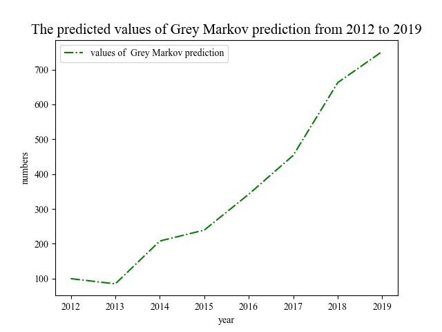
Based on the methods mentioned above, which involve the Grey Model and Markov correction chain, we conducted traditional Grey Markov prediction on the maintenance data of smart meters for a certain company in Wuhan, as shown in Table 1, covering the years 2012 to 2019. By fitting the data from the first 8 years, we constructed a traditional Grey Markov model and applied it to predict the data for the years 2020 to 2022 to assess its predictive accuracy. The total number of smart meters in this batch was 27,000.

Table 1. Maintenance Data for Smart Meters in a Wuhan Company

Using the Grey Model:

,,,,,,,

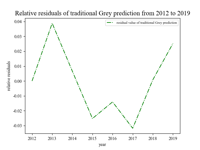
Based on the establishment of the traditional Grey prediction model as described in section 2.2, relative residuals ε_(k) were obtained, as shown in Figure 1. These residuals were divided into three corresponding state intervals: [-0.031, -0.0075], [-0.0075, 0.016], and [0.016, 0.0395], following the Markov chain correction method outlined in section 3.2. This yielded the predicted values of the Grey Markov model, which are presented in Table 2.

Table 2. Predicted Values by the Traditional Grey Markov Model

6. Fault Prediction with Grey Markov Model and Weakened Buffer Operator

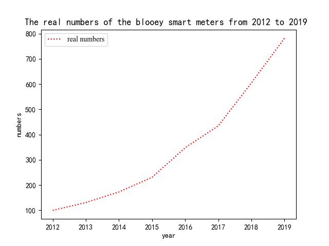
Figure 3. Actual Fault Data for Smart Meters from 2012 to 2019

Analyzing the data in Figure 3, it is evident that there was a relatively smooth increase in faults from 2012 to 2015, followed by an upward trend from 2015 to 2019. To achieve precise prediction for fault data from 2020 to 2022, it is essential to weaken the influence of earlier variations and enhance the contribution of new information. The introduction of the weakened buffer operator effectively achieves this and reduces prediction errors.

Utilizing the weakened buffer operator and the Markov correction chain methods described earlier, we conducted fault prediction with the Grey Markov model while applying the weakened buffer operator to the data in Table 1. We constructed a sequence after processing with the weakened buffer operator.

,,,,

The aforementioned sequence was subjected to level ratio testing, and it was found that it did not fall within the allowable coverage interval X. To address this, a translation process was applied, resulting in the sequence:

_,,_,,,

Using the least squares method, we obtained a = -0.085 and b = 1089.4. The GM(1,1) grey differential equation was transformed into the corresponding white differential equation:

(15)

This allowed us to calculate:

(16)

Through a reverse transformation of the buffer operator sequence, the corresponding predicted values were deduced:

,,,

By substituting the relative residual values ε_(k) into the Markov chain and applying the necessary residual correction, we obtained the corrected predicted values. Finally, subtracting the translation factor c = 1000 yielded the ultimate practical predicted values in Table 3.

Table 3. Predicted Values with Weakened Buffer Operator Grey Markov Model

The predicted values were subjected to error testing, and the accuracy levels are presented in Table 4. The original sequence’s variance was s₁², and the average relative error was p=0.0647, falling within the third level of accuracy. The correlation coefficient λ was calculated as the discrimination coefficient, taken as 0.5. Thus:

(17)

Where ε_min and ε_max represent the minimum and maximum residual values of the prediction results, respectively:

(18)

G falls within the third level of accuracy:

(19)

Where Δ ₍₀₎(k) represents the residual of the prediction results, and s₁² is the variance of the original sequence.

Table 4. Accuracy Levels

7. Establishment of Combination Models Based on the IOWA Operator and Fault Prediction

By comparing the correlation coefficient G and average relative error p, it is apparent that the Grey Markov model with the weakened buffer operator, as discussed previously, falls into the third level of accuracy and is not ideal for predictions. To further enhance the model’s predictive accuracy, this paper adopts the Induced Ordered Weighted Averaging (IOWA) operator’s combination forecasting method. This method assigns weights in order of the predictive accuracy of each individual forecasting method for sample points. The combination prediction is based on the criterion of minimizing the sum of squared errors [15, 16].

7.1. Establishment of the Combination Model Based on the IOWA Operator

The actual data sequence is denoted as x, and its value at time t is x_t. We consider m possible individual forecasting methods for x, and let x_it represent the predicted value for the i-th forecasting method at time t. Furthermore, a_it represents the prediction accuracy of the i-th forecasting method at time t. We define:

\( {a_{it}}=\begin{cases} \begin{array}{c} 0, when |\frac{{x_{t}}-{x_{it}}}{{x_{t}}}| \gt 1 \\ 1-|\frac{{x_{t}}-{x_{it}}}{{x_{t}}}|, when |\frac{{x_{t}}-{x_{it}}}{{x_{t}}}|≤1 \end{array} (i=1,2,…m, t=1,2,….,N)\end{cases} \) (20)

W=(w1, w2, …, n) as an ordered weighted average vector for various forecasting methods in the combination prediction. We arrange the forecasting methods based on their prediction accuracy, and x_a-index(it) represents the predicted value corresponding to the i-th prediction accuracy for time t. Therefore, the predicted value based on the IOWA operator at time t is given by:

(21)

Here, e_a-Index(it)=x_t-x_a-Index(it) and the total sum of squares can be calculated as:

(22)

Let, be the induced ordered weighted average combination prediction error information matrix. Therefore, the induced ordered weighted average combination prediction model can be expressed as follows:

(23)

This allows us to calculate the optimal weight coefficients and obtain the unique solution for the model.

7.2. Fault Prediction with the Combination Model Based on the IOWA Operator

Following the establishment process of the combination model based on the IOWA operator as described above, we can substitute the weakened buffer operator Grey Markov model and the Grey Markov model into the error information matrix [17, 18]:

(24)

As a result, the combination prediction model is given by:

(25)

We get . This model provides the corresponding predicted value, as presented in Table 5, and the error values are presented in Table 6. Visualization of the results can be seen in Figure 4.

Table 5. Predicted Values for Various Models

Table 6. Error Values for Various Models

The combined prediction model underwent post-analysis, yielding P=0.0306, which is in the second accuracy level, and G=0.821, also in the second accuracy level. Thus, the combined prediction model elevates the accuracy levels of P and G by one level.

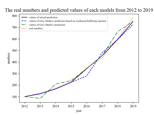
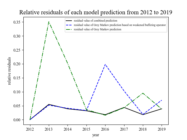
From the prediction chart, it can be deduced that the Grey Markov model with the weakened buffer operator exhibits high accuracy in the early stages but has some fluctuations in the middle and later stages. In contrast, the Grey Markov model displays higher fluctuations in the early stages but better fits the data in the middle and later stages. However, the combined model leverages the strengths of both models, making better use of existing data resources. Through training, it can provide more accurate predictions for smart meter fault data. Therefore, this combined model is chosen to predict the fault counts for smart meters in 2020 to 2022, as shown in Table 7.

Table 7. Predicted Smart Meter Fault Counts for 2020-2022 by Various Models

Analysis of the average relative error p indicates that the combination prediction outperforms the individual models’ predictions.

In summary, the process for predicting smart meter fault counts is illustrated in Figure 6.

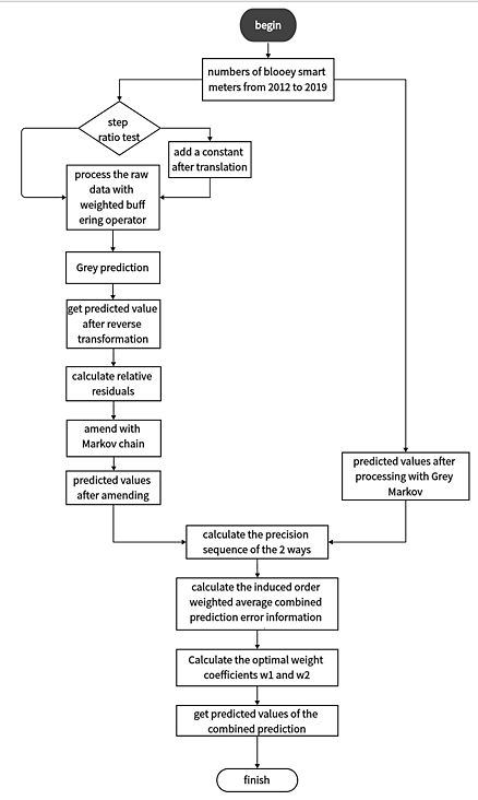
Figure 6. Flowchart of Smart Meter Fault Count Prediction Process

8. Conclusion

In summary, for the fault prediction of smart meters with limited information, a comprehensive comparison of posterior error p, C, and correlation coefficient G indicates that the combination model has distinct advantages. Therefore, the combined Grey Weakened Buffer Markov model based on the IOWA operator, compared to the methods in the literature [19-20], significantly improves prediction accuracy, enabling more precise medium- to long-term fault predictions. Through an overall prediction of the number of faults, this method can reveal potential issues and fault trends for smart meters. For instance, the growth trend in fault data can be used to assess whether the batch of meters meets quality standards. Predictive data for the coming year can be used to estimate the power supply instability and economic losses resulting from meter faults and maintenance, thereby providing data support for decisions on whether to replace this batch of meters or implement comprehensive meter maintenance. For example, by accurately predicting the number of faults, a company can make informed decisions on the allocation of maintenance personnel and fault handling resources, formulate relevant maintenance plans and strategies, proactively procure necessary spare parts and equipment, reduce prolonged power outages and energy losses due to faults, and subsequently improve the reliability and stability of the power grid. This approach plays a crucial role in guiding the maintenance of smart meters.

References

[1]. Liu Kaixin,Qi Jia,Zhou Zhen, et al.Multistate time lag dynamic Bayesian networks model for reliability prediction of smart meters [J] Microelectronics Reliability.Volume 138,Issue.2022.
[2]. Tao Peng,Shen Hongtao,Zhang Yangrui,et al.Research on the Life Prediction Method of Meters Based on a Nonlinear Wiener Process [J] Electronics.Volume 11 ,Issue 13.2022
[3]. Liang, Q. Y. (2023). Analysis and replacement management of intelligent electricity meter life prediction with the integration of electricity and environmental data [Doctoral dissertation, Dongbei University of Finance and Economics].
[4]. Huang, J. T., Fan, B., Zhou, Y. F., et al. (2019). Intelligent electricity meter fault and life prediction model based on random forest. Bing Gong Zi Dong Hua, 38(10), 57-60.
[5]. Wen, Y. K., Hou, H. J., Wang, Y. (2022). Intelligent electricity meter fault prediction based on Apriori and C5.0 algorithms. Zi Dong Hua Yi Biao, 43(05), 90-94+101.
[6]. Li, N., Zhang, W., Guo, Z. L., et al. (2022). Intelligent electricity meter fault prediction based on multi-class machine learning models. Dian Qi Yu Neng Xiao Guan Ji Shu, 2022(02), 6-11.
[7]. Gao, W. J., Xue, B. B., Pang, Z. J. (2022). Intelligent electricity meter fault prediction based on spatiotemporal convolutional neural networks. Dian Zi Ji Shu Ying Yong, 48(03), 59-63.
[8]. Fan, S. H. (2018). Research on intelligent electricity meter fault prediction technology based on big data analysis [Doctoral dissertation, Beijing University of Posts and Telecommunications].
[9]. Yang, J. C., Jiang, P., Chen, G. Y., et al. (2017). Research on intelligent electricity meter fault identification model. Dian Qi Yu Neng Xiao Guan Ji Shu, 2017(06), 30-36.
[10]. Jin Shuo Liu;Xin He;Shao Teng Li etc.Vertical Analysis Based on the Fault Data of Running Smart Meter.[J] Applied Mechanics and Materials.Volume 2370,Issue 313-314.
[11]. Liu, S. F. (2010). Grey system theory and its applications (5th ed.). Nanjing Hangkong Hangtian University.
[12]. Dang, Y. G., Liu, S. F., Liu, B., et al. (2004). Research on weakening buffer operator. Zhong Guo Guan Li Ke Xue, 2004(02), 109-112.
[13]. Huang, Y. S., Wang, F. F. (2013). Grey prediction based on weighted buffer operator. Dian Zi Ce Shi, 2013(20), 56-57.
[14]. Liu Sifeng, Deng Julong. The range suitable for GM (1,1)[J].Systems Engineering-Theory & Practice,2000, (5):121-124.
[15]. Ren, Y. J. (2023). Research on combination prediction model based on VIKOR-IOWA operator [Doctoral dissertation, Beijing Jiaotong University].
[16]. Zhang, Y. F. (2018). Combination prediction model based on IOWA operator under uncertain information [Doctoral dissertation, Anhui University].
[17]. Guo, L. J., Zhang, J. H. (2022). Wheat yield prediction based on combination of IOWA operator and grey neural network. Liang Shi Yu You Zhi, 35(10), 26-30.
[18]. Zhai, W. H. (2018). Improvement and application of grey Markov combination prediction model [Doctoral dissertation, Xi’an University of Architecture and Technology].
[19]. Wu, Z. M., Li, S. H., Wu, Y., et al. (2021). Consistency analysis of intelligent electricity meter accelerated degradation mechanism based on grey theory. Wuhan Da Xue Xue Bao (Gong Xue Ban), 54(11), 1070-1076.
[20]. Zhang, L. P., Hu, S. S., Mei, N., et al. (2020). A review of reliability research on intelligent energy meters. Dian Ce Yu Yi Biao, 57(16), 134-140.
Cite this article
Li,Z.;Xu,J. (2023). Smart meter failure prediction based on weakened grey markov model with IOWA operator. Theoretical and Natural Science,25,100-111.
Data availability
The datasets used and/or analyzed during the current study will be available from the authors upon reasonable request.
Disclaimer/Publisher's Note
The statements, opinions and data contained in all publications are solely those of the individual author(s) and contributor(s) and not of EWA Publishing and/or the editor(s). EWA Publishing and/or the editor(s) disclaim responsibility for any injury to people or property resulting from any ideas, methods, instructions or products referred to in the content.
About volume
Volume title: Proceedings of the 3rd International Conference on Computing Innovation and Applied Physics
© 2024 by the author(s). Licensee EWA Publishing, Oxford, UK. This article is an open access article distributed under the terms and
conditions of the Creative Commons Attribution (CC BY) license. Authors who
publish this series agree to the following terms:
1. Authors retain copyright and grant the series right of first publication with the work simultaneously licensed under a Creative Commons
Attribution License that allows others to share the work with an acknowledgment of the work's authorship and initial publication in this
series.
2. Authors are able to enter into separate, additional contractual arrangements for the non-exclusive distribution of the series's published
version of the work (e.g., post it to an institutional repository or publish it in a book), with an acknowledgment of its initial
publication in this series.
3. Authors are permitted and encouraged to post their work online (e.g., in institutional repositories or on their website) prior to and
during the submission process, as it can lead to productive exchanges, as well as earlier and greater citation of published work (See
Open access policy for details).