1. Introduction

Lung, bronchus and trachea cancers collectively pose a substantial public health challenge, with a staggering number of lives lost annually. In the United States, the year 2022 witnessed a daunting surge in cancer cases, with 1,918,030 new diagnoses reported. A sobering projection indicates that 609,360 individuals are anticipated to succumb to cancer, reflecting a profound societal impact, characterized by an alarming average of approximately 350 daily lung cancer-related fatalities, which is the leading cause of cancer deaths [1]. Evidently, lung cancer stands as the foremost cause of cancer-related deaths, emphasizing the urgent need for an intensified focus on prevention, early detection, and innovative treatment strategies. Lung cancer management has witnessed a shift, marked by significant strides in early detection methods and treatment modalities. These advancements, spanning recent decades, underscore a global commitment to combating this formidable disease [2]. Notably, the multifaceted nature of lung cancer necessitates a comprehensive understanding of its etiological factors and the implementation of diverse therapeutic interventions. Conventional treatments, including chemotherapy, surgical resection, and radiation therapy, have been instrumental in addressing lung cancer [3]. Crucially, the intricate tapestry of lung cancer etiology unravels various causative strands, notably encompassing smoking, lifestyle factors, genetic predisposition, dietary habits, occupational exposures, and ambient air pollution [4].

The trajectory of lung cancer, once a rarity 150 years ago, has witnessed a remarkable transformation, evolving into a prominent public health challenge over the ensuing decades. Several historical events, including World War I, the pervasive tobacco epidemic, and the rapid industrialization of societies, have collectively contributed to the substantial rise in the prevalence and mortality rates of lung cancer [5]. Understanding the evolution of this malignancy necessitates a meticulous analysis of its mortality rates across temporal epochs. Previous investigations have shed light on the emergence of lung cancer as a 20th-century epidemic in the United States, reaching its zenith towards the century’s closure. Fortunately, subsequent years have witnessed a reversal of this trend, marking a significant decline in the lung cancer epidemic, a trend that persists to the present day [6]. This dynamic landscape of lung cancer epidemiology has been a focal point of extensive research endeavors, particularly concerning future trends. Scholars and researchers have dedicated their efforts to forecasting the trajectory of lung cancer, thereby facilitating the development of innovative technologies aimed at early detection and, consequently, enhanced prevention strategies. Numerous studies have meticulously calculated and analyzed the incidence, mortality, and prevalence rates of lung cancer across various countries. These analyses have not only gauged the impact of lung cancer on populations but have also delved into the intricacies of the incidence rate formula, contributing valuable insights to the broader understanding of the disease’s epidemiological implications [7].

The analysis of lung cancer mortality rates serves as a pivotal endeavor, essential for enhancing the understanding, control, and prediction of this pervasive and deadly disease. Notably, advancements in screening methods have played a significant role in mortality reduction, exemplified by low-dose computed tomography (LDCT) screening, which has demonstrated the potential to decrease lung cancer mortality by up to 20% [8]. However, the limitations associated with LDCT, such as high false positive rates and associated risks, have propelled the exploration of alternative, non-invasive screening tools. Among these, long noncoding RNAs (lncRNAs) have emerged as promising candidates, offering accessibility and affordability in blood analysis, thus providing a more viable avenue for early detection and monitoring of lung cancer [9]. Moreover, this study builds upon prior research that categorized individuals into distinct groups based on smoking status, namely smokers, past smokers, and current smokers. Utilizing multivariate regression analysis and considering multiple risk factors, these datasets were meticulously scrutinized. In a departure from conventional approaches, this study delves into the striking disparity observed in lung cancer mortality rates between genders. Recognizing the significance of this gender-based difference, the analysis focuses specifically on delineating the mortality rates among men and women, thereby offering a nuanced perspective on the complexities of lung cancer epidemiology [10]. Furthermore, the endeavor to predict future trends in lung cancer mortality has been a subject of extensive research. However, limitations in the available annual data sample size restrict the scope of meaningful long-term predictions. To address this, this paper employs the R language, facilitating a robust analysis of the data. This method not only enables visualization of the data but also provides clear and unambiguous graphical representations, enhancing the precision of lung cancer mortality rate analysis. By leveraging computational tools, this research aims to shed light on the multifaceted dynamics of lung cancer mortality rates so that can pave the way for informed strategies and interventions.

2. Methods

2.1. Data source

The data presented in this literature pertains to age-standardized mortality rates for males and females in the US (per 100,000 people) due to lung, bronchus, and trachea cancer. The variable time span covers the years 1950 to 2020. The data was published by the World Health Organization, and the source of the publication date is the WHO Mortality Database. This paper accessed the data from the Our World in Data website, retrieved on May 16, 2022.

2.2. Method introduction

In this paper, the analytical approach involves the utilization of R to conduct a comprehensive analysis of the lung, bronchus, and trachea cancer death rates in the United States, specifically focusing on both male and female populations. Two distinct analytical models are employed in this investigation: the AutoRegressive Integrated Moving Average (ARIMA) model and the Exponential Smoothing State Space (ETS) model. These models are chosen for their efficacy in time series analysis, allowing for the exploration of temporal patterns and trends within the mortality data. The segmentation of the analysis into male and female death rates is a strategic methodological choice, driven by the noticeable disparity observed in the mortality rates between the genders. This demarcation enables a nuanced examination of the unique trajectories experienced by males and females in the context of lung-related cancers.

3. Results and discussion

3.1. ARIMA model

In this section, this paper employed the ARIMA model to meticulously dissect the dataset. Initially, the original data was visually represented through histograms, providing insightful glimpses into the temporal patterns of lung, bronchus, and trachea cancer death rates among males and females in the United States. For male lung-related cancer mortality rates, a discernible upward trajectory was evident from 1950 to 1990, followed by a significant downward trend from 1990 to 2020, indicating notable fluctuations over the decades. This is clear that the data are non-stationary, underscoring the necessity for further analytical treatment (Figure 1). Conversely, the histogram depicting female lung, bronchus, and trachea cancer death rates revealed a nuanced pattern. Between 1950 and 1960, there was a gradual, albeit slow, increase in mortality rates. Subsequently, from 1960 to 2000, a substantial upward trend was observed. Post-2000, a distinct downward trajectory emerged (Figure 2). These intricate trends emphasize the complexity of gender-specific patterns in lung-related cancer mortality rates. Subsequent part will delve into the results of the ARIMA analysis, providing deeper insights into the evolving trends that have shaped the landscape of lung-related cancer mortality rates among males and females in the United States.

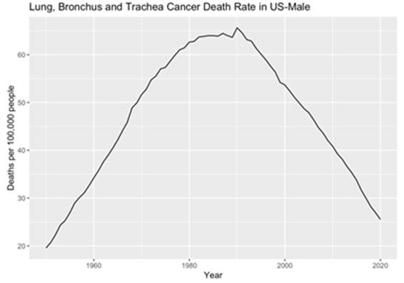
Figure 1. Male’s original data plot.

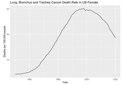
Figure 2. Female’s original data plot.

After the visual examination of the data, it became evident that the data were non-stationary, thus necessitating appropriate preprocessing methods for rigorous analysis. To address this, the dataset was subjected to differencing, resulting in the creation of two distinct data sets. This differentiating process ultimately yielded two stationary datasets for male and female lung, bronchus, and trachea cancer death rates (Figure 3 and 4). Meanwhile, through the application of the Augmented Dickey-Fuller test (ADF), the computed p-values for both male and female datasets were observed to be 0.01, indicating two stationary datasets and a high level of statistical significance. These results affirm the successful transformation of the datasets into stationary forms, laying the groundwork for subsequent in-depth analyses and ensuring the robustness of the findings presented in this study.

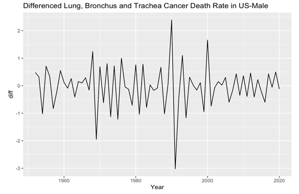
Figure 3. Male’s plot after differencing.

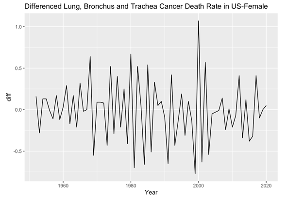
Figure 4. Female’s plot after differencing.

In the subsequent phase of the analysis, the Autocorrelation Function (ACF) and Partial Autocorrelation Function (PACF) plots were meticulously examined for both male and female death rates. These analytical techniques enabling the identification of significant correlations and dependencies within the data. Specifically, the histograms revealed that the male and female death rates exhibited non-white noise characteristics, as evidenced by the lags extending beyond the critical region (Figure 5, 6, 7 and 8). This notable deviation from white noise patterns underscores the presence of discernible temporal structures within the datasets, prompting a deeper exploration.

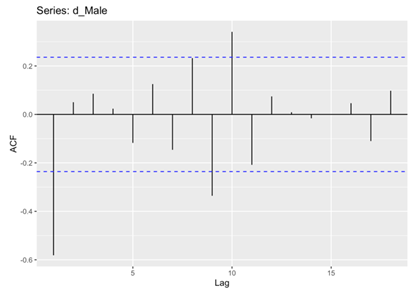
Figure 5. ACF for Male.

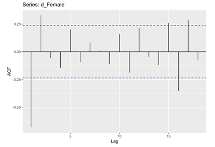
Figure 6. ACF for Female.

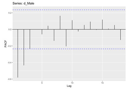
Figure 7. PACF for Male.

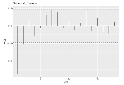
Figure 8. PACF for Female.

In the conclusive phase of the analysis, the AutoRegressive Integrated Moving Average (ARIMA) model was fitted to the preprocessed datasets (Table 1 and 2). To gauge the appropriateness of the models, two key metrics, namely the Akaike Information Criterion (AIC) and the Bayesian Information Criterion (BIC), were employed. AIC serves as a measure of the model’s goodness of fit, striking a balance between data fit and the avoidance of overfitting. Calculated using the formula AIC = 2k - 2ln(L) (where k represents the number of parameters and L is the likelihood function), models with lower AIC values are favored as they offer superior data fit while avoiding unnecessary complexity. Similarly, the Bayesian Information Criterion (BIC) operates in a similar vein. The BIC formula, BIC = k * ln(n) - 2 * ln(L) (where k is the number of parameters, n represents the number of samples, and L is the likelihood function). The value of BIC should be as small as possible and encouraging the selection of models that explain the data’s statistical characteristics.

Upon comparison of the AIC and BIC values for both male (AIC=125.83, AICc=126.45, BIC=134.76) and female (AIC=15.59, AICc=15.96, BIC=22.29), a discernible trend emerged. The AIC and BIC values derived from the female dataset were notably smaller than their counterparts from the male dataset. This discrepancy underscores the superior fit and explanatory power of the ARIMA models developed for the female dataset, indicative of a more precise representation of the underlying patterns.

Table 1. Fit ARIMA model for male’s data.

Table 2. Fit ARIMA model for Female’s data.

After applying the ARIMA models, residual checks were conducted for both male and female datasets to ascertain their adherence to the white noise assumption (Figure 9 and 10).

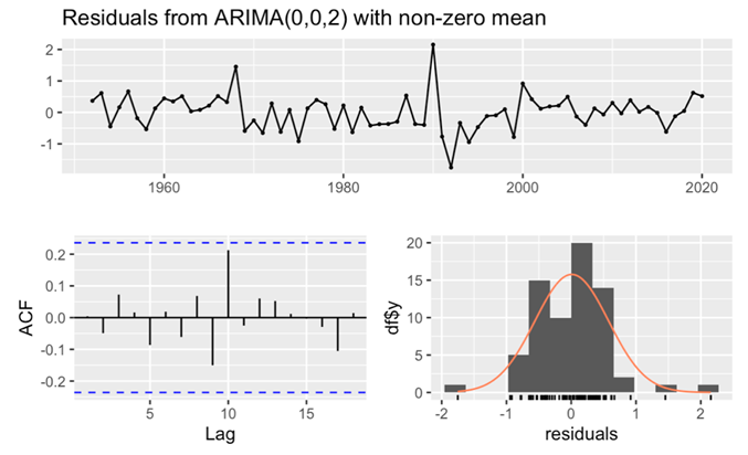
Figure 9. Residuals from ARIMA(0,0,2) for male’s data.

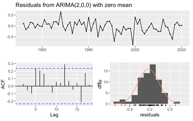
Figure 10. Residuals from ARIMA(2,0,0) for female’s data.

For the male dataset, the observation of a large p-value (larger than 0.05) (Table 3), in conjunction with all lags fell within the critical region of the ACF histogram, unequivocally confirmed the white noise nature of the residuals. This comprehensive analysis not only affirmed the adequacy of the model fit but also underscored its excellent goodness of fit, as meticulously recorded. Similarly, in the case of the female dataset, the p-value exceeding 0.05 (Table 4), coupled with the ACF histogram displaying nearly all lags within the critical region and the residuals histogram is normally distributed, corroborated the white noise characteristics of the residuals. These rigorous evaluations collectively affirmed the exceptional goodness of fit for the female dataset.

Table 3. Ljung-Box test for Male.

Table 4. Ljung-Box test for Female.

3.2. ETS model

In this section, the Exponential Smoothing State Space (ETS) model was employed to analyze both male and female death rates.

Firstly, focus on male death rate. Notably, the analysis of model parameters revealed that the parameter α closed to 1. The large level smoothing value (parameter α) means the recent observations have larger weight for forecasting. Contrarily, the parameter β not closed to 1. The small trend smoothing value (parameter β) means the forecast focuses on longer-term trend. Further scrutiny was directed towards the AIC and BIC values. The observed magnitudes of AIC and BIC are quite big and the model’s Mean Squared Error (MSE) value has a very small value (Table 5). This diminutive MSE value signifies a minimal forecasting error, underscoring the remarkable precision of the model. This underscores the model’s accuracy and efficacy, validating the robustness of the analytical approach and affirming the reliability of the outcomes derived.

Table 5. Fitting ETS for Male.

In the subsequent phase, this paper will analyze the components of ETS. From the histogram “Observed” represents the raw time series data which is the actual observations this paper needs to analyze and predict. “Level” represents the long-term average or trend in the time series data. It is usually an estimate of the trend component, which represents the direction of the long-term trend in the data. “Slope” is the magnitude of the change in the trend, i.e., whether the data is going up or down and at what rate. It represents the rate or rate of change of the long-term trend in the time series data. Upon analysis of the results, discernible patterns emerged from the histograms of both the Observed and Level components. An initial upward trend was observable, followed by a notable downward trajectory post-1990. Moreover, the Slope histogram depicted an overarching downward trend (Figure 11).

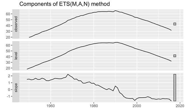
Figure 11. Components plot for male’s data.

In this part of the analysis, this paper turns the attention to the examination of residuals from the ETS model. This pivotal step aims to assess the adherence of residuals to the white noise assumption, providing critical insights into the model’s goodness of fit. The p-value notably exceeds 0.05, attesting to the model’s exceptional goodness of fit. Furthermore, a comprehensive analysis of the ACF shows a pattern wherein all spikes are within the critical interval. This spatial distribution affirms the absence of discernible correlations within the residuals, further bolstering the argument for the white noise nature of the residuals. In addition to the ACF examination, the histogram of residuals exhibits a distribution that adheres closely to the contours of a normal distribution. This adherence further fortifies the assertion that the residuals can be characterized as white noise (Figure 12).

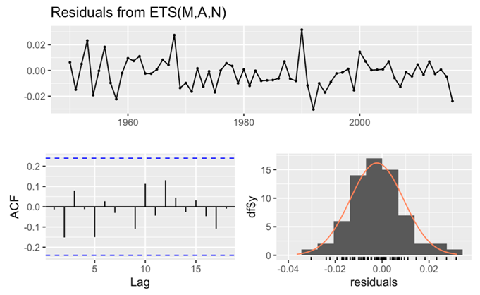
Figure 12. Checking the residuals for male’s data.

Secondly, focus on female death rate. In this part, this paper fitting the ETS model for female death rate. It shows the parameter α exhibited a close approximation to 1. Subsequently, an evaluation of the AIC and BIC values was performed. The observed diminutive values of AIC and BIC suggest a parsimonious model, indicative of an optimal balance between model complexity and explanatory power. Moreover, an assessment of the MSE revealed a diminutive value, emphasizing the model’s efficacy in minimizing forecasting errors. This diminutive MSE value attests to the model’s precision and accuracy in predicting the female death rate (Table 6).

Table 6. Fitting ETS for Female.

In the subsequent phase of the analysis, this paper direct the attention to the intricate components and residual characteristics derived from the ETS model. From the examination of ETS components, distinctive patterns emerge within the observed and level histograms. Initially, both histograms reveal an ascending trend until the year 2000, followed by a gradual descent thereafter. Similarly, scrutiny of the slope histogram unveils an upward trajectory from 1950 to 1980, succeeded by a subdued trend post-1980. These observations illuminate the dynamic interplay between long-term trends and fluctuations within the dataset. Then turning the attention to the check residuals. The p-value is greater than 0.05, attesting to the model’s outstanding goodness of fit. Additionally, the analysis of the ACF reveals that nearly all spikes fall within the critical interval. Further fortifying this assertion is the observation that the histogram of residuals adheres closely to a normal distribution, a characteristic indicative of white noise (Figure 13). In summation, these rigorous evaluations affirm the white noise nature of the residuals, affirming the model’s precision and its aptness in capturing the inherent patterns within the female death rate data.

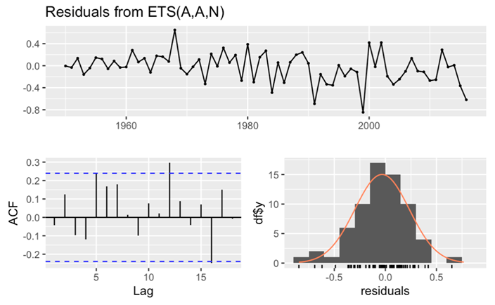
Figure 13. Checking the residuals for female’s data.

4. Conclusion

In conclusion, through the meticulous application of ETS and ARIMA models to the dataset, the discernment of white noise in the final results substantiates the efficacy of the models in capturing the inherent complexities of lung cancer mortality rates. Despite the stark gender disparity in lung cancer mortality, with men exhibiting significantly higher rates, the rising trend in women’s mortality rates necessitates sustained attention and proactive measures. The pervasive impact of lung cancer, attested by its high mortality rates, underscores its status as a global health challenge. The comprehensive analysis of annual data facilitates a nuanced understanding of the dynamic fluctuations in lung cancer trends. Leveraging historical data for predictive analyses not only aids in comprehending yearly variations but also empowers proactive measures for mortality rate control. In the ongoing quest for improved public health, sustained dedication to anti-smoking initiatives, robust air quality management, innovative screening and treatment programs and advancements in medical interventions collectively pave the way toward the eventual control of lung cancer mortality rates. It is an earnest hope that these multifaceted efforts will yield positive outcomes, contributing to the overarching goal of effectively curbing the impact of lung, bronchus and trachea cancers on global health.

References

[1]. Siegel R L, et al. 2021 Cancer statistics. Ca Cancer J Clin, 71(1), 7-33.
[2]. Adjei A A 2019 Lung cancer worldwide. Journal of Thoracic Oncology, 14(6), 956.
[3]. Sharma P, et al. 2019 Emerging trends in the novel drug delivery approaches for the treatment of lung cancer. Chemico-biological interactions, 309, 108720.
[4]. Malhotra J, et al. 2016 Risk factors for lung cancer worldwide. European Respiratory Journal, 48(3), 889-902.
[5]. Witschi H 2001 A short history of lung cancer. Toxicological sciences, 64(1), 4-6.
[6]. Alberg A J, Brock M V and Samet J M 2005 Epidemiology of lung cancer: looking to the future. Journal of clinical oncology, 23(14), 3175-3185.
[7]. Dubey A K, Gupta U and Jain S 2016 Epidemiology of lung cancer and approaches for its prediction: a systematic review and analysis. Chinese journal of cancer, 35(1), 1-13.
[8]. Tammemägi M C 2018 Selecting lung cancer screen using risk prediction models-where do we go from here. Translational lung cancer research, 7(3), 243.
[9]. Chen Y, et al. 2021 The function of LncRNAs and their role in the prediction, diagnosis, and prognosis of lung cancer. Clinical and translational medicine, 11(4), e367.
[10]. Spitz M R, et al. 2007 A risk model for prediction of lung cancer. Journal of the National Cancer Institute, 99(9), 715-726.
Cite this article
Zhang,X. (2024). The research of analysis lung, bronchus and trachea cancer death rate in US. Theoretical and Natural Science,30,38-49.
Data availability
The datasets used and/or analyzed during the current study will be available from the authors upon reasonable request.
Disclaimer/Publisher's Note
The statements, opinions and data contained in all publications are solely those of the individual author(s) and contributor(s) and not of EWA Publishing and/or the editor(s). EWA Publishing and/or the editor(s) disclaim responsibility for any injury to people or property resulting from any ideas, methods, instructions or products referred to in the content.
About volume
Volume title: Proceedings of the 3rd International Conference on Computing Innovation and Applied Physics
© 2024 by the author(s). Licensee EWA Publishing, Oxford, UK. This article is an open access article distributed under the terms and
conditions of the Creative Commons Attribution (CC BY) license. Authors who
publish this series agree to the following terms:
1. Authors retain copyright and grant the series right of first publication with the work simultaneously licensed under a Creative Commons
Attribution License that allows others to share the work with an acknowledgment of the work's authorship and initial publication in this
series.
2. Authors are able to enter into separate, additional contractual arrangements for the non-exclusive distribution of the series's published
version of the work (e.g., post it to an institutional repository or publish it in a book), with an acknowledgment of its initial
publication in this series.
3. Authors are permitted and encouraged to post their work online (e.g., in institutional repositories or on their website) prior to and
during the submission process, as it can lead to productive exchanges, as well as earlier and greater citation of published work (See
Open access policy for details).