1. Introduction

A bicycle-sharing system, bike share program [1], public bicycle scheme [2], or public bike share (PBS) scheme [3], is a shared transportation service, in which bikes can be provided to people at low prices. The plan itself includes a trailer system and a dock-free system, in which the trailer system allows users to rent bicycles from the dock, which is a technical bicycle box and return it to another node or dock in the system-there is no dock, providing an egg-free system based on intelligent technology. The system can integrate smart phone network map to locate available bicycles and docks. In July 2020, Google Maps began to include bike share systems in its recommendations of route [4].

The goal of this research is to not only develop a reliable prediction model but also through a comprehensive analysis of the dataset, this project seeks to unearth meaningful insights about the factors influencing bike rentals. These insights could potentially aid stakeholders in making informed decisions to optimize bike availability, marketing strategies, and resource allocation. The results of the study benefit customers as well because they can have an overview of the bike demand in each hour when they plan to rent one.

2. Literature Review

In the previous and present studies, there is much research on the prediction of bike-sharing demand, and most scientists use models to analyze and predict, some researchers use a single model to analyze and predict, while others choose multiple models and select the one with the best simulation effect to predict. Including Sathishkumar and other coauthors who used mining techniques, which contain Linear Regression, Gradient Boosting Machine, Support Vector Machine (Radial Basis Function Kernel), Boosted Trees, and Extreme Gradient Boosting Trees to evaluate target data to provide some ideas in solving the problem of making the rental bike available and accessible to the public at the right time as it lessens the waiting time [5]. Subsequently, Sathishkumar only used the Random forest model for bike-sharing demand prediction, he also had the conclusion that bike-sharing demand can be further improved by considering seasonal change [6]. Apart from only using the random forest model to predict, there are other examples of using a single model to predict like regression graph regularization [7], Low-Dimensional Model [8], etc. Sometimes the bike-sharing demand can be divided into more specific areas, such as the rental demand in different stations. This can also be predicted using the TAGCN model [9], and the idea of objectifying the demand in each station also provides more specific information about the bike-sharing service.

From the perspective of bike-sharing service, the amount of rentals is a key performance indicator for managers and supervisors in demand assessment. Therefore, the prediction of bicycle demand by bike-sharing system is a key index in economic system [10]. However, such prediction results can also benefit consumers with critical information. For example, people can anticipate the number of bike-sharing before renting it, which also dispels people's worries about not having enough bicycles to rent during peak hours to some extent. Also, trying to provide valuable information to bike-sharing services and their customers is not the only reason that leads to the study of prediction, there is research that is completed because of some problems including malicious damage, theft, chaotic parking, large-scale deficit, and bankruptcy [11].

Among the previous research, most of them are focusing on providing valuable information to the bike-sharing service system by using different types of methods. The differences between them are basically how specific is the demand—for example, in different stations or just the total number in an area—period of time(short-term or long-term), and different types of methods. It seems difficult to find some that used both machine learning to choose a model to predict and environmental elements, which will be the gap of this study.

To sum up, the research is going to focus on the prediction of bike sharing demand by hour using mostly environmental factors by linear regression, decision tree, and random forest.

3. Methodology

3.1. Data Description

This study selects a dataset which contains bicycles rented every hour in the Capital Bicycle Sharing System in Washington, D.C. from 2011 to 2012, and the corresponding climate and seasonal information.

Each factor’s detailed explanation in the selected dataset is listed in the appendix.

After the dataset is determined, three models are selected to analyze the data.

3.2. Linear Regression

Linear regression (LM) is equivalent to the connection between one or more X qualities of the input and the Y attribute of the scalar output. Simple linear regression is used when there are just one or two independent attributes, and multiple linear regression is used when there are several independent attributes.

It is relatively easy to use simple linear regression, which is a simple linear method for predicting a quantitative response Y based on just one predictor variable, X. It is predicated on the idea that X and Y have a roughly linear relationship. This linear relationship can be expressed mathematically as:

\( Y= {β_{0}}+ {β_{1}}X+ ε \) (1)

The \( ε \) stands for a mean-zero random error term, In the linear model, \( {β_{0}} \) and \( {β_{1}} \) , these two unknown constants stand in for the intercept and slope terms. Together, \( {β_{0}} \) and \( {β_{1}} \) are known as the model coefficients or parameters. After estimating \( \hat{{β_{0}}} \) and \( \hat{{β_{1}}} \) for the model coefficients using the training data, Y can be predicted based on a certain value of X by computing:

\( \hat{y}= \hat{{β_{0}}} \) and \( \hat{{β_{1}}}X \) (2)

where ˆy indicates a prediction of Y based on X = x.

In practical problems, \( {β_{0}} \) and \( {β_{1}} \) are unknown, therefore, before making predictions, estimating the coefficients by using the data is necessary.

The multiple linear regression’s method of application is similar to the simple linear regression, except with more than one independent variable. Therefore, the mathematical equation can be written as:

\( Y= {β_{0}}+ {β_{1}}{X_{1}}+ {β_{2}}{X_{2}}+ …+ {β_{p}}{X_{p}}+ ε \) (3)

One thing that must be made clear about linear regression is that the existence of correlation doesn’t mean the existence of causality. In other words, correlation in numerical statistics does not mean causality in practical problems, and the method is just responsible for dealing with the data, it should be carefully interpreted.

3.3. Decision Tree

Decision tree is a nonparametric supervised learning algorithm for classification and regression tasks. It has a hierarchical structure, a tree, which consists of root nodes, branches, internal ganglia and leaf nodes.

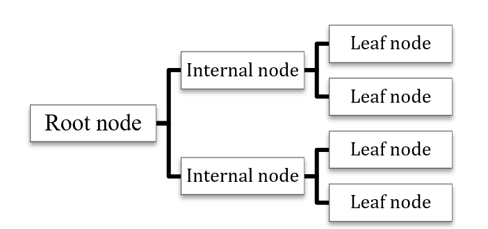
Figure 1. Basis of Decision Tree

As Figure 1 above shows, a decision tree begins with a root node that has no incoming branches. The internal nodes, also known as the decision nodes, are derived from the outgoing branches that from the root node. According to the available decision influencing factors, expand from the decision nodes, form homogeneous subsets, and finally get the leaf nodes or terminal nodes, which are the final decision results. The leaf nodes stand for all the possible results in the dataset. For instance, if you want to decide whether to go surf or not, the following decision rules can be used to make a choice:

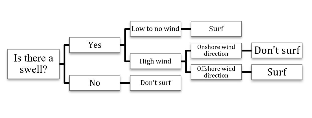
Figure 2. Decision Tree Sample

As the decision tree example shown in Figure 2, you need to consider different factors in each step and decide whether you want to go to surf or not. An easy-to-understand representation of decision-making is created by a flowchart structure such as this one, which helps various teams within the business better comprehend the reasoning behind decisions.

Decision tree learning uses attribution and conquest strategies to identify the best attribution points in the tree by performing Greek search. Then, this splitting process will be repeated and repeated until all (or most) documents are classified as specific class tags. Data points rely heavily on decision tree concurrency if they are all categorized as homogeneous sets. The data points in the nodesahuete, or class of the pure worksheet, are more easily accessible from smaller trees. But maintaining this purity gets harder and harder as the tree gets bigger, and most of the time, too much data is generated to fit into a single subtree. When this happens, it is called data fragmentation, which usually leads to over-utilization. Therefore, the decision tree is beneficial to young trees and conforms to the frugality principle of Occam’s Razor; In other words, "entities should not exceed necessity". That is to say, decision trees should only increase complexity when necessary, because the simplest explanation is usually the best. In order to reduce complexity and avoid over-assembly, pruning is usually used; this is a process of eliminating branches divided on low-importance features. Cross-validation can be used to assess model fitting. Creating a set using the random forest algorithm is another technique to preserve the accuracy of a decision tree; this classifier can forecast outcomes with greater accuracy, particularly in situations when individual trees are not connected to one another.

3.4. Random Forest

There are multiple decision trees in the random forest model.

Random forest algorithm has three main super parameters, which must be set before it is trained. These consist of the node's size, the number of trees, and the quantity of features that have been chosen. As a result, regression and classification issues can be resolved using the random forest classifier.

The random forest algorithm consists of a series of trees, each tree as a whole, and consists of data samples extracted from an alternative education package called "bootstrap". In this tutorial, one-third of them are placed as test data, called "out-of-bag(oob) samples". Another organization responsible for calibration is introduced through function package, which increases the diversity of data and reduces the proportion among decision trees. The certainty of the forecast will change because of the type of problem. For regression problems, a single decision tree will be an average, and for classification, most decision trees will be binary stars. The most common class variation will lead to the emergence of predefined classes. Finally, oob samples are used for cross-validation, which completes the prediction.

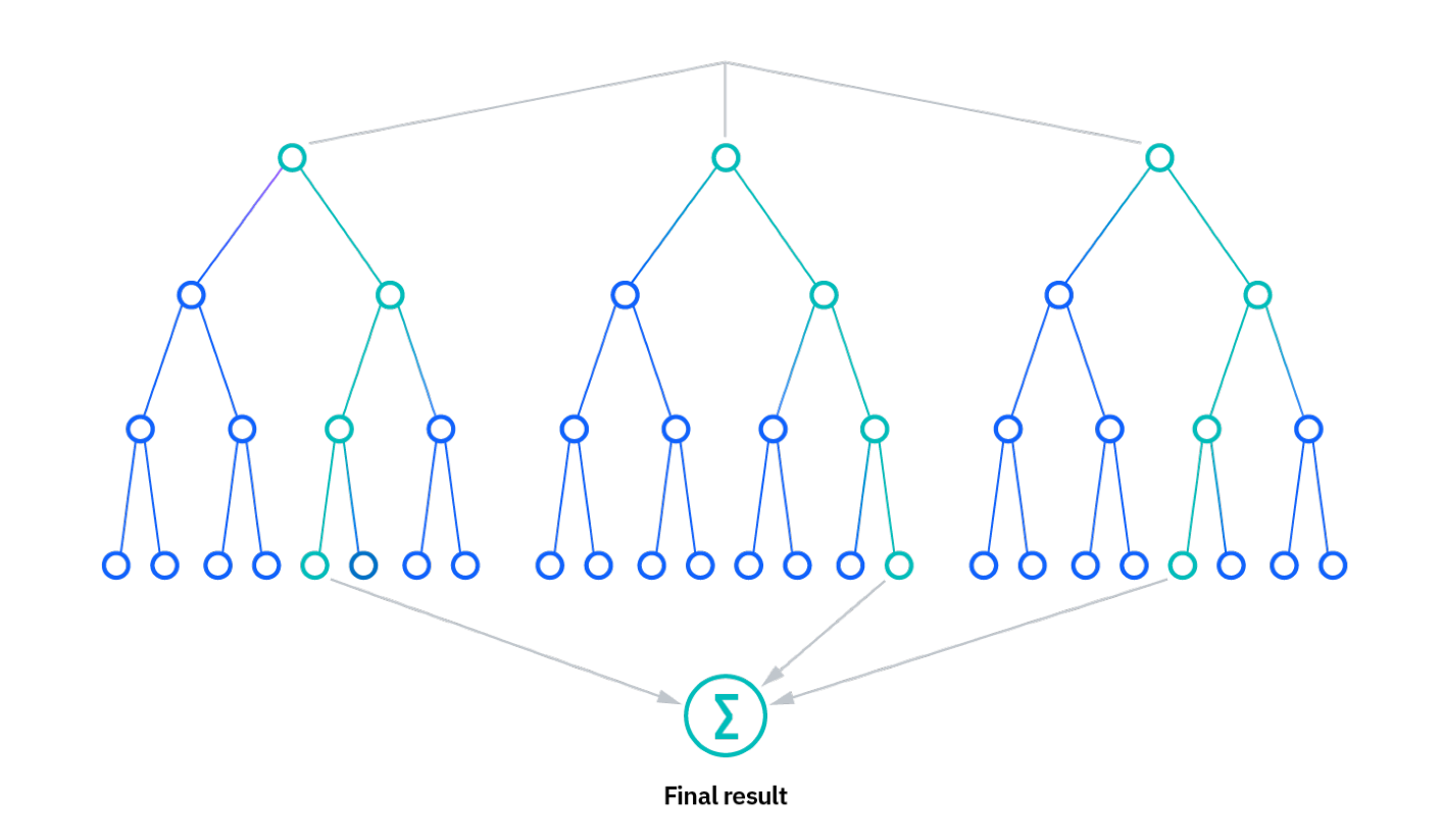
Figure 3. Random Forest Explanation

As Figure 3 shows, compared with the decision tree, the random forest model contains more points of view before making the final decision. For instance, like the surf example above, if someone wants to go surf the decision tree may only consider the factor “Is there a swell?”, but the random forest will include more elements such as “Are there too many people?” “Will I get hurt” and so on. That’s also why the random forest model contains several decision trees.

4. Results

In this research, the original data is separated into the training dataset and test dataset before analysis.

4.1. Processing the data

The first thing that I did in this research was restore qualitative data that was transferred into quantitative data in the training dataset, because as the data description mentioned in 3.1, there are some data like the season, holiday, working day, and weather sections are stored in numerical terms. It is better for analyzing to transfer them into qualitative terms. For example, “1” stands for Clear in whether section, therefore this step transfers it into “Clear” and then stores in the dataset, “0” stands for not holiday in the holiday section, so it is changed into “not holiday” in the dataset, so as other data like this one.

4.2. Appendix: Detailed Data Description

instant: Record Index

dteday: Date

season: Season (1:springer, 2:summer, 3:fall, 4:winter)

yr: Year (0: 2011, 1:2012)

mnth: Month (1 to 12)

hr: Hour (0 to 23)

holiday: weather day is holiday or not (extracted from Holiday Schedule)

weekday: Day of the week

workingday: If day is neither weekend nor holiday is 1, otherwise is 0.

weathersit: (extracted from Freemeteo)

1: Clear, Few clouds, Partly cloudy, Partly cloudy

2: Mist + Cloudy, Mist + Broken clouds, Mist + Few clouds, Mist

3: Light Snow, Light Rain + Thunderstorm + Scattered clouds, Light Rain + Scattered clouds

4: Heavy Rain + Ice Pallets + Thunderstorm + Mist, Snow + Fog

temp: Normalized temperature in Celsius. The values are derived via (t-t_min)/(t_max-t_min), t_min=-8, t_max=+39 (only in hourly scale)

atemp: Normalized feeling temperature in Celsius. The values are derived via (t-t_min)/(t_max-t_min), t_min=-16, t_max=+50 (only in hourly scale)

humidity(hum): Normalized humidity. The values are divided to 100 (max)

windspeed: Normalized wind speed. The values are divided to 67 (max)

casual: count of casual users

registered: count of registered users

cnt: count of total rental bikes including both casual and registered

4.3. Data Visualization and Analysis

4.3.1. Correlation Matrix. Before building the model, it need to have an intuitive understanding of the correlation between these numerical variables.

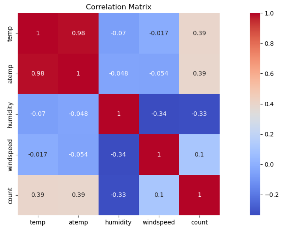
Figure 4. Correlation Matrix

Figure 4 illustrates that apart from temp and atemp has a high correlation, which is acceptable, because the feeling temperature has just slight differences with the real temperature, others are in the safe zone for analyzing.

4.3.2. Total Rental Demand in Different Types of Days. The number of total rental bikes can be different because the number of people outside will be different for different types of days.

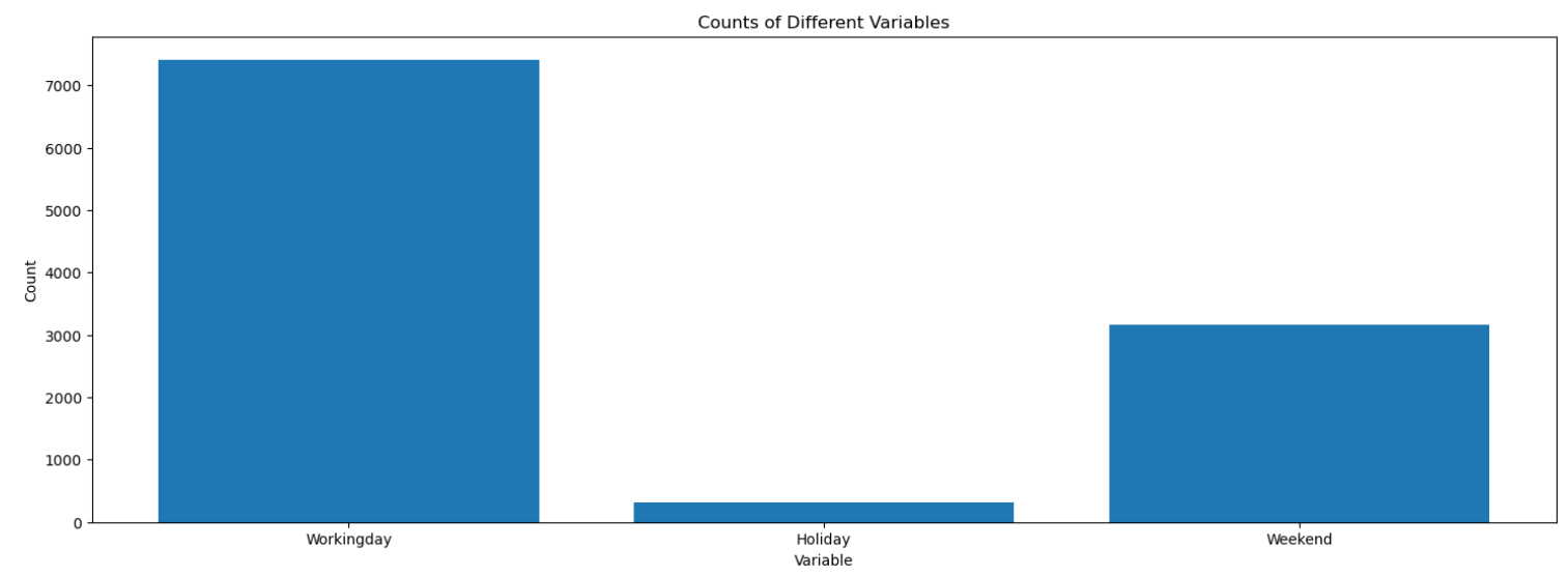
Figure 5. Counts of Different Variables

It can seen from Figure 5 that the total rental number of bikes is the largest on weekdays, followed by weekends, then holidays.

4.3.3. Average Rental Counts by Hours of the Day. The number of total rental bikes can be different because the number of people outside will be different for different types of days.

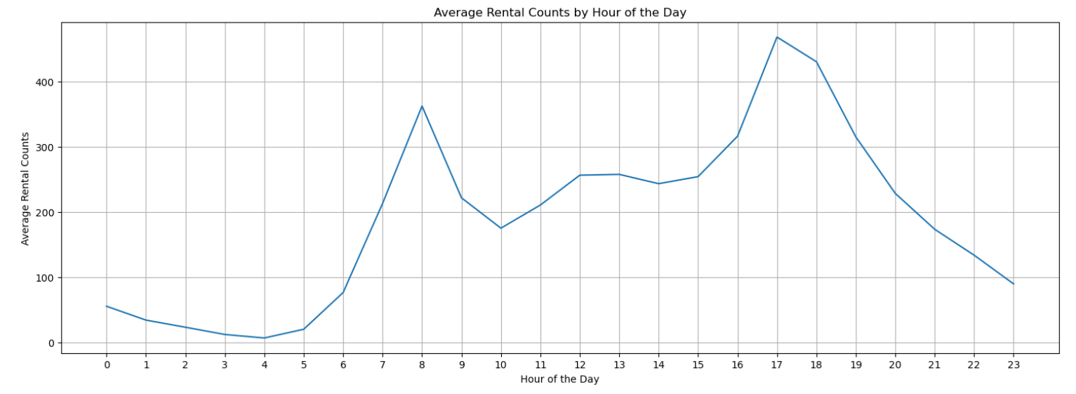
Figure 6. Average Rental Counts by Hour of the Day

From Figure 6 it can get the information that 7:00 to 9:00 and 16:00 to 19:00 are two peak hours that have the second largest and largest rental number respectively. In other periods of the day, people rent the most bikes in the afternoon, followed by evening and early morning.

4.3.4. Average Rental Counts by Hour on each day of the Week

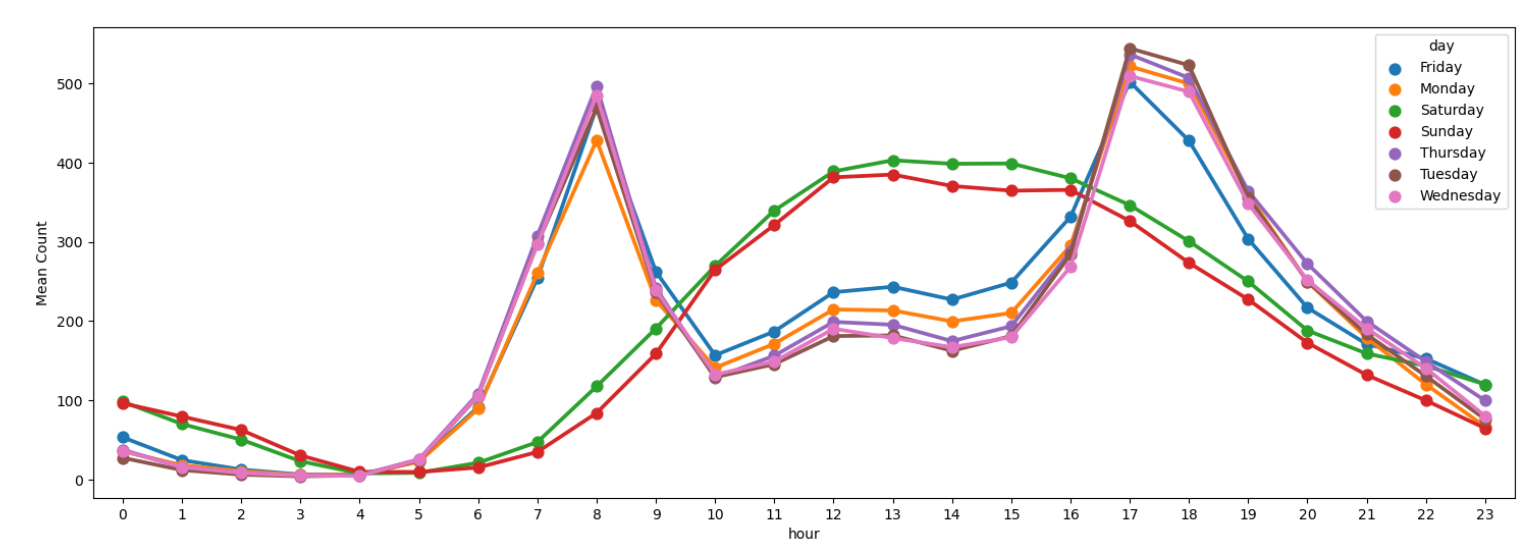
Figure 7. Average Rental Counts by Hour on each day of the Week

Figure 7 shows that the trend of the number of average rentals in bike-sharing is different on weekends and working days, but the trend of days on weekends and working days is the same.

4.3.5. Average Rental Counts by Season

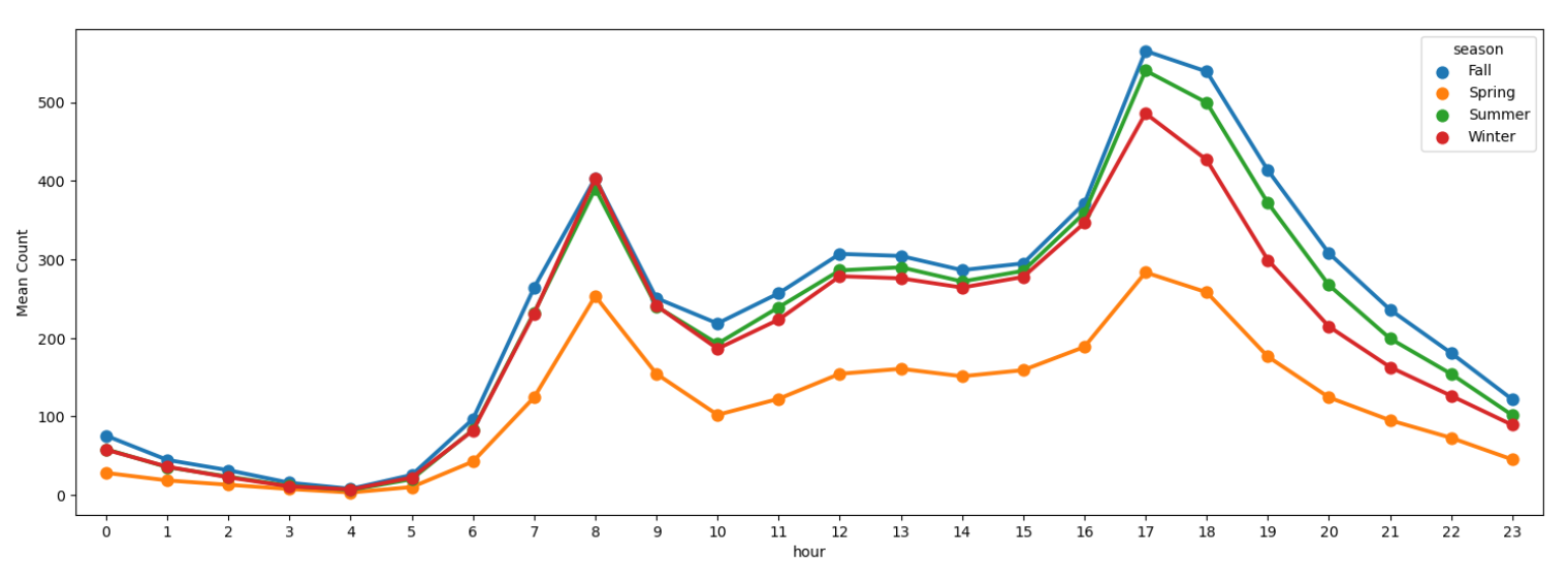
Figure 8. Average Rental Counts by Season

Figure 8 above shows that the average rental bike number has a similar trend through four seasons. Also, people rent the most in fall, although in winter at 8:00 took its position, followed by summer, winter, and spring.

4.4. Modeling

The Root Mean Squared Logarithmic Error (RMSLE) scorer is utilized to assess the model's performance. RMSLE is a metric commonly used in regression tasks to measure the accuracy of predictions. It penalizes underestimation and overestimation of the target variable, making it suitable for this bike rental count prediction task. The lower the RMSLE value, the better the model's predictions align with the actual target values.

4.4.1. Evaluate Different Regression Models Using Cross-Validation

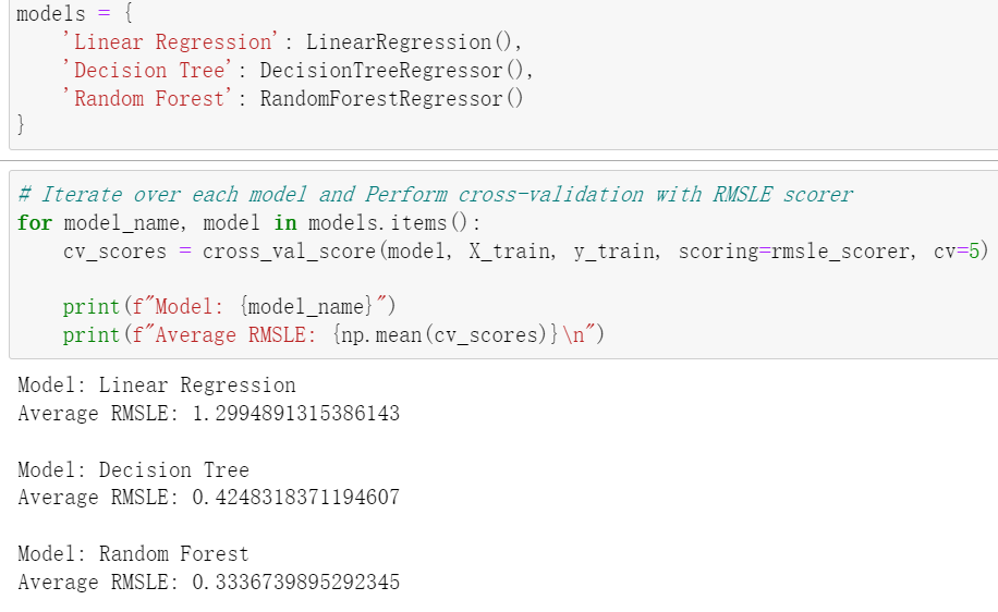
Figure 9. Model Evaluation Results

As shown in Figure 9, after evaluating multiple regression models, the Random Forest algorithm demonstrated the best performance based on the RMSLE metric. Therefore, this paper selected the Random Forest model to make predictions on the test data.

5. Conclusion

This study first improves the data set through detailed steps, including date-time format conversion, classification value replacement, and solving anomalies in variables such as humidity and wind speed. These basic works have laid the foundation for more accurate analysis and model training. (Some steps not shown in the article will be shown in the code file.)

Through exploratory data analysis, the study has revealed important trends and patterns. It is observed that the number of bike rentals on weekdays exceeds that on weekends and holidays, and certain peak hours continue to attract more rentals.

In the model evaluation, the random forest algorithm shows extraordinary ability by obtaining the lowest RMSLE score, so it is selected as the prediction model in the future.

In conclusion, this research contains data extraction, profound analysis, meticulous model selection, and comprehensive utilization of prediction. This effort has provided valuable strategic decision-making information for both producers and consumers in bike-sharing. Therefore, the producers should provide more bikes in peak hours, and also use different bike demand-providing strategies in working days, holidays, and weekends since they have different trends. As for customers, if it’s hard to avoid the peak hours when the work time is fixed, then it’s more valuable to consider the period when it’s a more flexible situation, such as hanging out on working days or going out on weekends.

Another interesting conclusion this study comes to is how to choose between RMSLE and R-squared. Both RMSLE and R-squared quantify the adaptability of linear regression model to dataset. The RMSLE shows the degree to which the regression model can predict the value of the response variable in absolute value while R-squared shows to what extent the predicted variables can explain the changes of the response variables. In this research, the author was in the situation of choosing the best prediction model, which means RMSLE will be more suitable. The study focuses on the relationship between predictor variables and response variables, \( {R^{2}} \) .

In other words, RMSLE is more useful in choosing a better or the best model to predict, therefore it’s the comparison between different models, whereas \( {R^{2}} \) is normally used in one specific model analysis, such as its considerate function in multiple linear regression.

As for the limitation of this study, firstly, this prediction mainly used factors that are environmentally connected, such as humidity, temperature, and so on. However, there may be more elements influencing bike-sharing demand. For example, the brand of bike-sharing, the quality of the bike, the color of the bike, etc. It is not saying that increasing selected factors will certainly increase the possibility of prediction, but the research will be more convincing because of the cautious attitude.

References

[1]. "The Many Benefits of Bike Sharing Programs", 2016, (Commute Options), Retrieved 27 August 2021.
[2]. Kodukula, S. 2010, "Recommended Reading and Links on Public Bicycle Schemes", (European Commission), Retrieved 7 August 2019.
[3]. Mattlamy. 2019. "A guide to hire bikes and public bike share schemes", (Cycling UK).
[4]. Porter, J. 2020, "Google Maps now shows cycling routes using docked bike-sharing schemes", (The Verge), Retrieved 24 July 2020.
[5]. Sathishkumar, V. E. Jangwoo, P. Yong, Y. C. 2020, Using data mining techniques for bike sharing demand prediction in metropolitan city, (Computer Communications, vol. 153), pp. 353-366.
[6]. V, E. S. Cho, Y. 2020, Season wise bike sharing demand analysis using random forest algorithm, (Computational Intelligence), pp. 1-26.
[7]. Wang, X.D. Cheng, Z. H. Martin, T. Sun, L. J. 2021, Modeling bike-sharing demand using a regression model with spatially varying coefficients, (Journal of Transport Geography, vol. 93), no. 103059.
[8]. Cantelmo, G. Kucharski, R. Antoniou, C. 2020, Low-Dimensional Model for Bike-Sharing Demand Forecasting that Explicitly Accounts for Weather Data, (Transportation Research Record, vol. 2674), no. 8, pp. 132-144.
[9]. Zi,W. J. Xiong, W. Chen, H. Chen, L. 2021, Station-level demand prediction for bike-sharing system via a temporal attention graph convolution network, (Information Sciences, vol. 561), pp. 274-285.
[10]. Chang, P. C. Wu, J. L. Xu, Y. et al. 2019, Bike sharing demand prediction using artificial immune system and artificial neural network, (Soft Comput, vol. 23), pp. 613–626.
[11]. Xiao, G. Wang, R. Zhang, C. et al. 2021, Demand prediction for a public bike sharing program based on spatio-temporal graph convolutional networks, (Multimed Tools Appl, vol. 80), pp. 22907–22925.
Cite this article
Qian,X. (2024). Using machine learning for bike sharing demand prediction. Theoretical and Natural Science,30,110-119.
Data availability
The datasets used and/or analyzed during the current study will be available from the authors upon reasonable request.
Disclaimer/Publisher's Note
The statements, opinions and data contained in all publications are solely those of the individual author(s) and contributor(s) and not of EWA Publishing and/or the editor(s). EWA Publishing and/or the editor(s) disclaim responsibility for any injury to people or property resulting from any ideas, methods, instructions or products referred to in the content.
About volume
Volume title: Proceedings of the 3rd International Conference on Computing Innovation and Applied Physics
© 2024 by the author(s). Licensee EWA Publishing, Oxford, UK. This article is an open access article distributed under the terms and
conditions of the Creative Commons Attribution (CC BY) license. Authors who
publish this series agree to the following terms:
1. Authors retain copyright and grant the series right of first publication with the work simultaneously licensed under a Creative Commons
Attribution License that allows others to share the work with an acknowledgment of the work's authorship and initial publication in this
series.
2. Authors are able to enter into separate, additional contractual arrangements for the non-exclusive distribution of the series's published
version of the work (e.g., post it to an institutional repository or publish it in a book), with an acknowledgment of its initial
publication in this series.
3. Authors are permitted and encouraged to post their work online (e.g., in institutional repositories or on their website) prior to and
during the submission process, as it can lead to productive exchanges, as well as earlier and greater citation of published work (See
Open access policy for details).