1. Introduction

In 1887, Michelson and Morley identified the fine structure spectral lines [1]. However, this result does not coincide with the Bohr model of atom. Scientists have published their own revisions to quantum physics, which was still an incomplete discipline at that time. However, the contribution of Paul Dirac is the one mainly focused on this article. “The new quantum mechanics, when applied to the problem of the structure of the atom with point-charge electrons, does not give results in agreement with experiment” [2], said Paul Dirac, in the opening of his article The Quantum Theory of the Electron. The stationary states of an electron in atom were observed to be twice the number of that predicted by the theory considering electron as a point-charge. Dirac referred to it in his article by stating that, the discrepancy was created by the incompleteness of the previous theories lying in their disagreement with relativity. In his idea and as he proposed in his article, the simplest Hamiltonian for the electron would satisfy both relativity and general transformation theory and can solve all the duplexity phenomena without further assumptions. Nowadays, the extra energy levels observed were known to be caused by spin-orbit coupling, a relativistic-phenomenon between the spin of electron and its orbit around a nucleus. While this phenomenon was unknown to the world until 1928, it has become very popular in advanced investigation in not only the field of Quantum physics, but also in the field of materials, etc. For example, the research in spin-orbit coupling discovers the topological surface states, which can be applied to spin batteries [3]. In addition, research also indicates that when the tunnel barrier height is appropriately matched, the tunnel junction’s electrical conductivity exhibits a significant switching effect, [4] which would be beneficial for developments in electronics.

This article will provide a concise examination of the contributions made by Dirac’s theory to the refinement of atomic structure. To elucidate further, the paper will initially introduce essential terminologies such as electron, atomic structure, and spin-orbit coupling, followed by a derivation of Dirac’s equation. Subsequently, the article will delve into the application of Dirac’s equation to address the problem. In conclusion, the article will assess both the merits and constraints of Dirac’s theory.

2. Terminology and Theory

There are several important subjects in the article. They will be comprehensively described here to avoid complicated explanation in the later sections of this article.

2.1. Electrons, Spin, and Spin-Orbit Coupling

Electron is one of the most familiar fundamental particles in the Standard Model. Being different from photons which are classified as Bosons in the standard model, electrons, together with quarks, are Fermions, which are half-integer spins instead of integer spin like bosons does. Having negative one elementary electrical charge enables electrons to be attracted by atom nucleus and orbit around it. As mentioned in the above lines, electrons have half-integer spin, \( 1/2 \) -spin specifically. Spin is an intrinsic property possessed by elementary particles, and thus the composite particles such as atom nuclei, hadrons, etc. Literally, it would be misinterpreted as a rotating inertial mass, but it is in fact a quantized wave property. Spin was firstly inferred from Stern-Gerlach experiments, in which the sliver atoms were found to have two discrete angular momenta after passing through an inhomogeneous magnetic field, even though the atoms have no angular momentum in the first place [5]. In Figure 1, the pattern pointed by number 4 is the classical prediction. However, what obtained is the pattern pointed by 5.

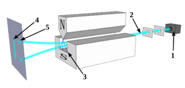
Figure 1. Simplified Display of Stern-Gerlach Experiment Setup

Atomic structure describes the orbits of electrons around the nucleus. Bohr’s quantized energy levels of orbiting electrons only makes up the Gross Structure of atom. In a more precise model, the Fine Structure, the spin of electrons is considered, resulting in splitting the gross structure spectral lines. In Figure 2, the two peaks demonstrate the split of electron energy in Chlorine \( p \) orbit, resulting in a splitting of the original energy state. The phenomenon is called the spin-orbit coupling.

As mentioned above, spin-orbit interaction is considered in the fine structure model of atomic structure. It is a relativistic effect which the spin of the electron is interacting with the magnetic field created by positively charged nucleus, breaking the degeneracy of gross structure energy levels. This interaction arises in fine structure but not in gross structure because only electric potential energy is considered. However, in the fine structure, the nucleus is moving and a moving charge at speed \( v \) with electric field \( E \) creates magnetic fields \( B=\frac{-v×E}{{c^{2}}} \) . With additional energy levels, spin-orbit interaction has its own Hamiltonian  \( {\hat{H}_{s-o}} \) as a perturbation to the original Hamiltonian. From the perspective of magnetic field and the physical relation behind it, \( {\hat{H}_{s-o}} \) can be directly derived as follows.

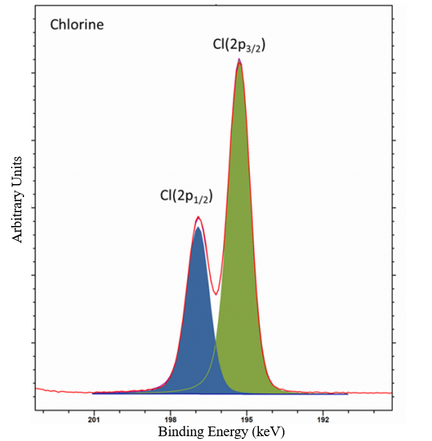
Figure 2. Energy splitting of electron caused by spin-orbit coupling in chlorine \( p \) orbit [6].

Given the gyromagnetic factor \( {g_{s}} \) , which is an add-on numerical relation, the Bohr magnetic, which is \( {μ_{B}}=\frac{eℏ}{2{m_{e}}} \) , and the magnetic dipole moment, which is proportional to spin, the magnetic dipole moment for electron is

\( μ=\frac{-e}{2{m_{e}}}\cdot L={g_{s}}\cdot \frac{-e}{2{m_{e}}}\cdot L=-{g_{s}}\cdot {μ_{B}}\frac{L}{ℏ}\ \ \ (1) \)

Turning the angular momentum of an electron into an operator would give the spin operator \( \hat{s} \) and the above relation would become

\( \hat{μ}=-{g_{s}}\cdot \frac{{μ_{B}}\hat{s}}{ℏ}≈-2{μ_{B}}\frac{\hat{s}}{ℏ}\ \ \ (2) \)

In Eq. (2), the \( -2 \) comes from the approximation of gyromagnetic factor \( {g_{s}}≈2.00231930437378(2) \) [7]. Now the spin-orbit Hamiltonian can be calculated by concerning both Larmor interaction \( {\hat{H}_{L}} \) and Thomas interaction \( {\hat{H}_{T}} \) .

Firstly, for Larmor interaction, the Hamiltonian can be written as \( {\hat{H}_{L}}=-{\hat{μ}_{B}}\cdot B \) . In this equation, magnetic field is given as \( B=-\frac{v×E}{{c^{2}}} \) . The dot product here implies that the energy depends on the alignment between the magnetic dipole moment and the magnetic field. To obtain the relation of \( v \) and \( E \) , rearranged equation of \( P={m_{E}}\cdot v \) and \( E=|E|\cdot \frac{r}{r} \) are used, and therefore \( B=-\frac{P}{{m_{e}}}×r\cdot \frac{E}{r}\cdot \frac{1}{{c^{2}}}=\frac{r×P}{{m_{e}}{c^{2}}}\cdot |\frac{E}{r}| \) . Since electric field strength \( E \) and electric potential \( V \) has relationship: \( E=-∇V \) . In addition, a central field approximation can be used for an electron in hydrogen atom. Therefore, \( |E| \) can be written as \( |E|=|\frac{∂V}{∂r}|=\frac{1}{e}\frac{∂U(r)}{∂r} \) . Therefore, the magnetic field now changes to \( B=\frac{1}{{m_{e}}{c^{2}}\cdot e}\cdot \frac{1}{r}\cdot \frac{∂U(r)}{∂r}\hat{l} \) . By substituting \( B \) into \( {\hat{H}_{L}} \) , the Hamiltonian for Larmor interaction is given by

\( {\hat{H}_{L}}=-\hat{μ}\cdot B≈-2{μ_{B}}\frac{\hat{s}}{ℏ}\cdot \frac{1}{{m_{e}}{c^{2}}e}\cdot \frac{1}{r}\cdot \frac{∂U(r)}{∂r}\cdot \hat{l}\ \ \ (3) \)

Now the Thomas interaction \( {\hat{H}_{T}} \) is considered, which gives the relation of \( {\hat{H}_{T}}={Ω_{T}}\cdot \hat{s} \) . In this relation, \( {Ω_{T}}=-ω(γ-1) \) . \( ω \) is the angular frequency of the electron and \( γ \) is the Lorentz factor. By putting the conditions of an electron in hydrogen atom into the equation gives

\( {\hat{H}_{T}}={Ω_{T}}\cdot \hat{s}=\frac{-{μ_{B}}}{4{m_{e}}e{c^{2}}}\cdot \frac{1}{r}\cdot \frac{∂U(r)}{∂r}\cdot \hat{l}\cdot \hat{s}\ \ \ (4) \)

Finally, the total spin-orbit Hamiltonian constitute of these two interactions, which gives the equation as \( {\hat{H}_{s-o}}={\hat{H}_{L}}+{\hat{H}_{T}} \) . Therefore, by adding them together and approximate the gyromagnetic factor to 2 gives

\( {\hat{H}_{s-o}}={\hat{H}_{L}}+{\hat{H}_{T}}≈\frac{{μ_{B}}}{ℏ{m_{e}}e{c^{2}}}\frac{1}{r}\frac{∂U(r)}{∂r}\cdot \hat{s}\cdot \hat{l}\ \ \ (5) \)

For a hydrogen atom, the electric potential is \( \frac{{e^{2}}}{r} \) . In this case, the spin-orbit Hamiltonian is in its complete form: \( {\hat{H}_{s-o}}=\frac{{e^{2}}}{2m_{e}^{2}{c^{2}}{r^{3}}}\cdot \hat{s}\cdot \hat{l} \) .

2.2. Theories and Dirac Equation

For a free particle, the Dirac equation can be written in the form of [8]

\( iℏ\frac{∂|Ψ⟩}{∂t}=(cα\cdot P+βm{c^{2}})|Ψ⟩.\ \ \ (6) \)

It can be proven by starting from Free-Particle Schrodinger Equation, which is

\( iℏ\frac{∂|Ψ⟩}{∂t}=\frac{{P^{2}}}{2m}|Ψ⟩\ \ \ (7) \)

To be consistent with relativity, the Hamiltonian \( \hat{H} \) should follow the energy equation from relativity, which is \( E=\sqrt[]{{c^{2}}{p^{2}}+{m^{2}}{c^{4}}} \) . Therefore,

\( \hat{H}={({c^{2}}{p^{2}}+{m^{2}}{c^{4}})^{\frac{1}{2 }}}\ \ \ (8) \)

Therefore, Eq. (7) would be changed to \( iℏ\frac{∂|Ψ⟩}{∂t}={({c^{2}}{p^{2}}+{m^{2}}{c^{4}})^{\frac{1}{2}}}|Ψ⟩ \) . However, this equation is undesired because space and time is treated asymmetrically, which can be shown by expanding the right-hand side of this equation in momentum basis:

\( iℏ\frac{∂|Ψ⟩}{∂t}={({c^{2}}{p^{2}}+{m^{2}}{c^{4}})^{\frac{1}{2}}}|Ψ⟩=m{c^{2}}(1+\frac{{p^{2}}}{2{m^{2}}{c^{2}}}-\frac{{p^{4}}}{8{m^{4}}{c^{4}}}+…).\ \ \ (9) \)

When transforming back to coordinate basis, each \( {p^{2}} \) becomes \( (-{ℏ^{2}}{∇^{2}}) \) , which is in second order. While on the left-hand side of Eq. (9), the time derivative is first order. To solve this problem, Eq. (8) can either be squared or changed. By squaring it, the corresponding energy equation would become \( \frac{{∂^{2}}|Ψ⟩}{∂{t^{2}}}=[-\frac{{c^{2}}{P^{2}}}{{ℏ^{2}}}-\frac{{m^{2}}{c^{4}}}{{ℏ^{2}}}]|Ψ⟩ \) . In coordinate basis it becomes \( [\frac{1}{{c^{2}}}\frac{{∂^{2}}}{∂{t^{2}}}-{∇^{2}}+{(\frac{m{c^{2}}}{ℏ})^{2}}]Ψ=0 \) . This equation is called the Klein-Gordon equation with desired symmetry between space and time. But the shortcoming is also manifest: \( Ψ \) here is a scalar and it cannot describe electron. The other way is to change the Hamiltonian by writing the quantity in the square root as a perfect square of a quantity that is linear in \( P \) . Therefore, Eq. (8) changes to

\( {c^{2}}{p^{2}}+{m^{2}}{c^{4}}={(c{α_{x}}{P_{x}}+c{α_{y}}{P_{y}}+c{α_{z}}P\_z+βm{c^{2}})^{2}}={(cα\cdot P+βm{c^{2}})^{2}}\ \ \ (10) \)

In this case, \( α \) and \( β \) can be determined by expanding the perfect square and matching the left-hand side of Eq. (10)

\( {c^{2}}(P_{x}^{2}+P_{y}^{2}+P_{z}^{2})+{m^{2}}{c^{4}}=[{c^{2}}(α_{x}^{2}P_{x}^{2}+α_{y}^{2}P_{y}^{2}+α_{z}^{2}P_{z}^{2})+{β^{2}}{m^{2}}{c^{4}}] \)

\( +[{c^{2}}{P_{x}}{P_{y}}({α_{x}}{α_{y}}+{α_{y}}{α_{x}})+{c^{2}}{P_{y}}{P_{z}}({α_{y}}{α_{z}}+{α_{z}}{α_{y}})+{c^{2}}{P_{z}}{P_{x}}({α_{z}}{α_{x}}+{α_{x}}{α_{z}})] \)

\( +m{c^{3}}[{P_{x}}({α_{x}}β+β{α_{x}})+{P_{y}}({α_{y}}β+β{α_{y}})+{P_{z}}({α_{z}}β+β{α_{z}})]\ \ \ (11) \)

For this equation to equal \( {c^{2}}{p^{2}}+{m^{2}}{c^{4}} \) , the following relation must be true: \( α_{i}^{2}={β^{2}}=1 \) , \( {α_{i}}{α_{j}}+{α_{j}}{α_{i}}=0={[{α_{i}},{α_{j}}]_{+}} \) , and \( {α_{i}}β+β{α_{i}}=0={[{α_{i}},β]_{+}} \) , in which \( i≠j \) and \( i j ∈\lbrace xyz\rbrace \) . In this case, the value of \( α \) and \( β \) can be obtained as \( α=[\begin{matrix}0 & σ \\ σ & 0 \\ \end{matrix}] \) and \( β=[\begin{matrix}I & 0 \\ 0 & -I \\ \end{matrix}] \) .

3. Coupling Electron to a Potential

In this section, the Dirac equation (see Eq. (6)) derived above will be used to calculate certain cases of potential when an electron is coupled to. In this way, two properties of electron can be shown to emerge very naturally from Dirac’s theory. The two properties are: 1. The value of gyromagnetic factor \( {g_{s}} \) for electron and the spin-orbit Hamiltonian \( {\hat{H}_{s-o}} \) .

To couple an electron to a potential \( (A,ϕ) \) , the Hamiltonian of Dirac equation should be modified to include potential energy and the change of kinetic energy due to the potential. Therefore, the Hamiltonian will be changed to \( \hat{H}={[{(P-q\frac{A}{c})^{2}}{c^{2}}+{m^{2}}{c^{4}}]^{\frac{1}{2}}}+q \) . By substituting this into the Dirac equation would give: \( iℏ\frac{∂Ψ}{∂t}=[cα\cdot (P-q\frac{A}{c})+βm{c^{2}}+qϕ] \) . In this equation, the value of \( A \) and \( ϕ \) are determined by each case to be analysed.

3.1. Gyromagnetic Factor \( {g_{s}} \)

The condition for potential in this case is: \( ϕ=0 \) and work to the order of \( {(\frac{v}{c})^{2}} \) . If the eigenstates of electron \( Ψ(t)=Ψ\cdot {e^{-i\frac{E}{tℏ}}} \) in this case is desired, then the energy eigenstate equation can be written as

\( EΨ=(cα\cdot π+βm{c^{2}})\ \ \ (12) \)

in which \( π=P-\frac{qA}{c} \) is the kinetic momentum of the electron. Rearrange and expanding the matrix \( α \) and \( β \) in Eq. (12) would give the following equation:

\( [\begin{matrix}E-m{c^{2}} & σ\cdot π \\ σ\cdot π & E+m{c^{2}} \\ \end{matrix}]\ \ \ (13) \)

In this equation, the wavefunction \( Ψ \) can be written as a matrix composed of Dirac spinors so that it can be expressed as: \( Ψ= [\begin{matrix}χ \\ Φ \\ \end{matrix}] \) . Therefore, Eq. (13) can be written as

\( [\begin{matrix}E-m{c^{2}} & σ\cdot π \\ σ\cdot π & E+m{c^{2}} \\ \end{matrix}][\begin{matrix}χ \\ Φ \\ \end{matrix}]=0.\ \ \ (14) \)

Implicating the basic matrix multiplication would give two relations:

\( (E-m{c^{2}})χ-cσ\cdot πΦ=0\ \ \ (15) \)

\( (E+m{c^{2}})Φ-cσ\cdot πχ=0\ \ \ (16) \)

Rearranging Eq. (16) would give the following relation:

\( (\frac{cσ\cdot π}{E+m{c^{2}}})χ=Φ.\ \ \ (17) \)

The denominator of the LHS of Eq. (17) is \( E+m{c^{2}}={E_{s}}+2m{c^{2}} \) , in which \( {E_{s}}=E-m{c^{2}} \) is the energy appears in Schrodinger Equation and it also equations to \( {E_{s}}=\frac{{π^{2}}}{2m}+V \) . According to virial theorem, \( {E_{s}} \) can be approximated to \( {E_{s}}≈m{v^{2}} \) . Therefore, \( \frac{{E_{s}}}{m{c^{2}}}≈{(\frac{v}{c})^{2}}≪1 \) at low velocity and the denominator can therefore be approximated to be \( E+m{c^{2}}={E_{s}}+2m{c^{2}}≈2m{c^{2}} \) . Therefore, substituting the approximated value of the denominator into Eq. (17) would give \( Φ≈\frac{cσ\cdot π}{2m{c^{2}}}χ=\frac{σ\cdot π}{2mc}χ \) . And by substituting Eq. (13) into Eq. (15) would give

\( {E_{s}}χ-cσ\cdot πΦ=0\ \ \ (18) \)

\( {E_{s}}χ=cσ\cdot π\cdot \frac{σ\cdot π}{2mc}χ=\frac{(σ\cdot π)(σ\cdot π)}{2m}χ=\frac{{(σ\cdot π)^{2}}}{2m}\ \ \ (19) \)

By using the identity: \( (α\cdot A)\cdot (α\cdot B)=A\cdot B+iσ\cdot A×B \) and \( π×π=\frac{iqℏ}{c}B \) , Eq. (19) would be

\( [\frac{{(P-\frac{qA}{c})^{2}}}{2m}-\frac{qℏ}{2mc}σ\cdot Bχ]={E_{s}}\ \ \ (20) \)

Eq. (20) describes a spin-1/2 particle with a gyromagnetic factor \( {g_{s}}=2 \) . It is manifest that only the condition of the potential is given to the Dirac equation and the value of \( {g_{s}} \) can be naturally obtained from Dirac’s theory. By considering the radiative corrections, experimental result from CODATA provides a more precise correction to \( {g_{s}}≈2.00231930436256(35) \) [7]. This correction can be calculated by considering the relative change in the electron magnetic dipole moment in the first order of expansion \( \frac{δμ}{μ}=\frac{{g_{s}}}{2}-1=\frac{{e^{2}}}{2πℏc} \) . By substituting \( \frac{{e^{2}}}{ℏc}=\frac{{e^{2}}}{e_{*}^{2}} \) [9], where \( {e_{*}} \) is the coupling charge, \( \frac{δμ}{μ}=\frac{1}{2π}\frac{{e^{2}}}{e_{*}^{2}}=\frac{α}{2π} \) . In this equation, \( α=\frac{{e^{2}}}{e_{*}^{2}}=\frac{1}{137} \) is the fine structure constant. Therefore, \( \frac{{g_{s}}}{2}-1=0.001162 \) , which gives \( {g_{s}}=2.002324 \) . Utilizing a higher order of expansion would yield a significantly more accurate alignment with the experimental value.

3.2. Spin-Orbit Coupling revisited

The condition for the spin-orbit interaction of an electron in a hydrogen atom is: \( V=eϕ=\frac{-{e^{2}}}{r} \) , which is a typical central field. In this case, the proton is approximated to be fix and it is infinitely massive compared to the mass of an electron. For this case, an energy eigenstate equation is also desired. Therefore, like the writing of Eq. (12), the energy eigenstate equation can be written as \( (E-V)Ψ=(cα\cdot P+βm{c^{2}})Ψ \) in this case. In the same way, this equation can also be separated into two relations of Dirac spinors \( χ \) and \( Φ \) [10]:

\( (E-V-m{c^{2}})χ-cσ\cdot PΦ=0\ \ \ (21) \)

\( (E-V+m{c^{2}})Φ-cσ\cdot Pχ=0\ \ \ (22) \)

Eq. (22) can be rearranged to the form of \( Φ=\frac{cσ\cdot P}{E-V+m{c^{2}}} \) . Substituting \( Φ \) in Eq. (21) can give

\( (E-V+m{c^{2}})χ=c(σ\cdot P)\cdot \frac{cσ\cdot P}{E-V+m{c^{2}}}.\ \ \ (23) \)

By approximating \( E-V+m{c^{2}}≈2m{c^{2}} \) would only give the typical Schrodinger equation in the form of \( {E_{s}}χ=(\frac{{(σ\cdot P)^{2}}}{2m}+V) \) . This is because the approximation is made under the circumstance of low speed, which is just the non-relativistic conditions. To further calculate and obtain the Hamiltonian in the energy eigenstate equation, \( \frac{1}{E-V+m{c^{2}}} \) is expanded. Thus,

\( \frac{1}{E-V+m{c^{2}}}=\frac{1}{2m{c^{2}}+{E_{s}}-V}=\frac{1}{2m{c^{2}}}{(1+\frac{{E_{s}}-V}{2m{c^{2}}})^{-1}}≈\frac{1}{2m{c^{2}}}(1-\frac{{E_{s}}-V}{2m{c^{2}}})\ \ \ (24) \)

and

\( \frac{1}{E-V+m{c^{2}}}≈\frac{1}{2m{c^{2}}}-\frac{{E_{S}}-V}{4{m^{2}}{c^{4}}}.\ \ \ (25) \)

Therefore, substituting this expansion into Eq. (23) gives

\( {E_{s}}χ=[\frac{{P^{2}}}{2m}+V-\frac{σ\cdot P({E_{s}}-V)σ\cdot P}{4{m^{2}}{c^{2}}}],\ \ \ (26) \)

which is obviously not an energy eigenstate function because the energy term \( {E_{s}} \) appears at both side of the equation. Hence, to eliminate \( {E_{s}} \) , \( ({E_{s}}-V)σ\cdot P \) is expanded as

\( ({E_{s}}-V)σ\cdot Pχ=σ\cdot P({E_{s}}-V)χ+σ\cdot [{E_{s}}-V,P]=(σ\cdot P)\frac{{P^{2}}}{2m}χ+σ\cdot [P,V]\ \ \ (27) \)

Substituting the expanded form into Eq. (26) gives the energy eigenstate equation desired:

\( {E_{s}}χ=\lbrace \frac{{P^{2}}}{2m}+V-\frac{{P^{4}}}{8{m^{3}}{c^{2}}}-\frac{iσ\cdot P×[P,V]}{4{m^{2}}{c^{2}}}-\frac{P\cdot [P,V]}{4{m^{2}}{c^{2}}}\rbrace χ=\hat{H}χ.\ \ \ (28) \)

In this way, the total Hamiltonian for an electron in hydrogen atom is obtained in the energy eigenstate equation for this case. Notice that there are five terms in the Hamiltonian and each of them have their own contribution. Firstly, \( \frac{{P^{2}}}{2m} \) is in a very typical form and it contributes to the kinetic energy. Secondly, \( V \) is the term that contributes to the potential energy. Thirdly, \( -\frac{{P^{4}}}{8{m^{3}}{c^{2}}} \) is the relativistic correction to the electron kinetic energy due to the high travelling speed of electron in this case. Fourthly, \( -\frac{iσ\cdot P×[P,V]}{4{m^{2}}{c^{2}}} \) is the spin-orbit Hamiltonian term. It can be expanded as: \( -\frac{iσ\cdot P×[P,V]}{4{m^{2}}{c^{2}}}=-\frac{iσ\cdot P×[-iℏ∇(\frac{-{e^{2}}}{r})]}{4{m^{2}}{c^{2}}}=\frac{-ℏ{e^{2}}σ\cdot P×r}{4{m^{2}}{c^{2}}}=\frac{ℏ{e^{2}}}{4{m^{2}}{c^{2}}{r^{3}}}σ\cdot r×P \) . Therefore, \( {\hat{H}_{s-o}}=\frac{{e^{2}}}{2{m^{2}}{c^{2}}{r^{3}}}\cdot \hat{s}\cdot \hat{l} \) . In this expansion, with the properties of \( r×P=L \) and \( σ=\frac{2\hat{s}}{ℏ} \) , it is manifest that the obtained spin-orbit Hamiltonian is the same as the one derived previously. Finally, \( -\frac{P\cdot [P,V]}{4{m^{2}}{c^{2}}} \) is known as the Darwin term.

4. Conclusion

In this article, Dirac equation is utilized to solve for two cases of potential coupled which electron is coupled to, aiming to prove the comprehensiveness of Dirac equation as a modification of quantum mechanics for electrons and atomic fine structure. In the case of \( ϕ=0 \) , the Dirac equation is found to be naturally fits the electron theories and gives an electron gyromagnetic factor of \( {g_{S}}=2 \) . Considering first order radiative correction to it, \( {g_{s}} \) can be in closer proximity to the experimental value, giving \( {g_{s}}=2.002324 \) . On the other hand, when considering the spin-orbit coupling with a central field of \( V=\frac{-{e^{2}}}{r} \) , the obtained spin-orbit Hamiltonian from Dirac equation is the same as the one calculated from the physical relations considering Larmor and Thomas interaction. These two cases show the superiority of Dirac’s theory dealing with spin- \( 1/2 \) particles such as electron and the success of Dirac in solving the duplexity at the time. The achievement of Dirac in explaining atomic fine structure and spin-orbit coupling is crucial for the development of corresponding technologies using these theories. As an illustration, investigations into spin-orbit coupling have unveiled topological surface states that have potential applications in spin batteries. Furthermore, studies have revealed that by precisely aligning the height of the tunnel barrier, significant switching effects in the electrical conductivity of tunnel junctions can be achieved, a finding with promising implications for advancements in the field of electronics. The Dirac equation, while consistent with the principles of special relativity, demonstrates limited applicability in the presence of strong external fields, making it only valid in weak external fields situations, such as the electron’s orbital motion around a nucleus. Furthermore, it remains incongruent with the broader framework of general relativity. Thus, efforts are still required to solve the challenge of unifying quantum field theory with the principles of general relativity.

References

[1]. Michelson A. A. and Morley E. W. (1887). On the relative motion of the earth and the luminiferous aether. Philosophical Magazine Series 5, 24: 449-463.
[2]. Dirac Paul. A. M. (1928). The quantum theory of the electron. Proceedings of the Royal Society of London. Series A, Containing Papers of a Mathematical and Physical Character, 117: 778.
[3]. Soumyanarayanan A., et al. (2016). Emergent phenomena induced by spin–orbit coupling at surfaces and interfaces. Nature, 539(7630): 509-517.
[4]. Yang Jun, Dai Bingfei. Li Xia. (2011). Spin orbit coupling effect and its application. College Physics, 30(8): 2-4.
[5]. Schmidt L., Lüdde H. J., Trageser W., Templeton A., Sauer T., Schmidt-Böcking, H. (2016). The stern-gerlach experiment revisited. The European Physical Journal H, 41(4-5): 327-364.
[6]. Lee, S.-H., Liu, K. (1999). Exploring the spin–orbit reactivity in the simplest chlorine atom reaction. The Journal of Chemical Physics, 111(14): 6253-6259.
[7]. Hajhamed Diab, et al. (2023). A comparative study of the solutions of the Klein-Gordon and Dirac equations: Implications for particle physics. EPRA International Journal of Research and Development (IJRD), 80(2): 78.
[8]. Shankar R. (2014). Principles of Quantum Mechanics, Second Edition, Springer, 564-565.
[9]. Gao Feng, Zong Zhi-wen (2018). The Lande Factor of j-j Coupling, Journal of Hengyang Normal University, 3(39): 43-46.
[10]. Daywitt William C. (2019). The dirac equation and its relationship to the fine structure constant according to the plank vacuum theory. Progress in Physics, 15(2): 55-57.
Cite this article
Bai,D. (2024). Dirac equation and its contribution to atomic fine structure. Theoretical and Natural Science,30,133-140.
Data availability
The datasets used and/or analyzed during the current study will be available from the authors upon reasonable request.
Disclaimer/Publisher's Note
The statements, opinions and data contained in all publications are solely those of the individual author(s) and contributor(s) and not of EWA Publishing and/or the editor(s). EWA Publishing and/or the editor(s) disclaim responsibility for any injury to people or property resulting from any ideas, methods, instructions or products referred to in the content.
About volume
Volume title: Proceedings of the 3rd International Conference on Computing Innovation and Applied Physics
© 2024 by the author(s). Licensee EWA Publishing, Oxford, UK. This article is an open access article distributed under the terms and
conditions of the Creative Commons Attribution (CC BY) license. Authors who
publish this series agree to the following terms:
1. Authors retain copyright and grant the series right of first publication with the work simultaneously licensed under a Creative Commons
Attribution License that allows others to share the work with an acknowledgment of the work's authorship and initial publication in this
series.
2. Authors are able to enter into separate, additional contractual arrangements for the non-exclusive distribution of the series's published
version of the work (e.g., post it to an institutional repository or publish it in a book), with an acknowledgment of its initial
publication in this series.
3. Authors are permitted and encouraged to post their work online (e.g., in institutional repositories or on their website) prior to and
during the submission process, as it can lead to productive exchanges, as well as earlier and greater citation of published work (See
Open access policy for details).