1.Introduction

Hydrogen is the simplest element in the universe and plays a vital role in scientific research. It has only one proton and one electron structure, making it an excellent subject for many preliminary studies to understand the fine structure of atoms. Theoretically, its simple structure enables accurate comparisons between theoretical and experimental results. For a long time, people have been trying to construct a model of the hydrogen atom but without success, until the advent of quantum mechanics [1].

In the early 20th century, quantum mechanics revolutionized people’s understanding of atoms. Quantum mechanics believes that energy has the smallest unit, rather than being absolutely continuous. Hydrogen’s simple atomic structure made it a major subject of early quantum research. The Schrödinger equation for hydrogen is a very important step in connecting quantum ideas to actual atomic structure. Through the Schrödinger equation, scientists explained the distribution of its electrons and the characteristics of its spectrum. Through theoretical calculations, physicists also explained the splitting of spectral lines in magnetic fields [2]. There is a question that many people are thinking about: Will the spectral lines of hydrogen atoms also split under an electric field? In fact, this phenomenon exists. External electric fields have the ability to change atomic energy levels, a phenomenon known as the Stark effect. The Stark effect is one of the key discoveries in the history of quantum mechanics. It provides a direct method for studying the energy level structure of atoms and molecules. This effect helps physicists verify the basic principles and predictions of quantum mechanics and gain a deeper understanding of how electrons within atoms respond to external electric fields. The Stark Effect has many practical applications. For example, the Stark effect, in which an external electric field changes the energy levels of atoms, is used in technologies from lasers to semiconductors. The high-frequency Stark effect of hydrogen and helium spectral lines can be used for plasma diagnosis [3]. Molecules containing vibrational Stark shift reporters can be used to measure DC electric fields in situ [4]. The perturbation generated by the Stark effect will affect the frequency of atomic clocks, and scientists are trying to solve this effect [5].

This article will discuss hydrogen starting with basic quantum theory and reviewing the discovery of the Stark effect. and further research into the Stark effect, emphasizing its importance in historical and contemporary physics.

2.Physical Basis of Hydrogen Atom

2.1.Wave Function of Hydrogen Atom

The Schrodinger’s equation in 3D is expressed as

\( -\frac{{ℏ^{2}}}{2m}{∇^{2}}ψ(\vec{r})+V(r)ψ(\vec{r})=Eψ(\vec{r})\ \ \ (1) \)

where\( ℏ \)is reduced plank’s constant,\( m \)is the mass of the electron,\( {∇^{2}} \)is Laplacian operator,\( V(\vec{r}) \)is the potential of the system (Coulomb potential), and\( E \)is the energy of the system. Since the hydrogen atom in 3D is a sphere, it is better to solve Schrodinger’s equation under spherical coordinates. Transform to spherical coordinates\( \vec{r}=(r,θ,ϕ) \), it is found that

\( {∇^{2}}=\frac{1}{{r^{2}}}\frac{∂}{∂r}({r^{2}}\frac{∂}{∂r})+\frac{1}{{r^{2}}sin{(θ)}}\frac{∂}{∂θ}(sinθ\frac{∂}{∂θ})+\frac{1}{{r^{2}}{sin^{2}}θ}\frac{{∂^{2}}}{∂ϕ},\ \ \ (2) \)

and thus

\( -\frac{{ℏ^{2}}}{2m}[\frac{1}{{r^{2}}}\frac{∂}{∂r}({r^{2}}\frac{∂ψ}{∂r})+\frac{1}{{r^{2}}sin{θ}}\frac{∂}{∂θ}(sinθ\frac{∂ψ}{∂θ})+\frac{1}{{r^{2}}{sin^{2}}θ}\frac{{∂^{2}}ψ}{∂ϕ}]+V(r)ψ(r,θ,ϕ)=Eψ(r,θ,ϕ)\ \ \ (3) \)

Then use separation of variables to break the equation. Suppose\( ψ(r,θ,ϕ)=R(r)Y(θ,ϕ) \)and substitute this back to Eq (3),

\( -\frac{{ℏ^{2}}}{2m}[\frac{Y}{{r^{2}}}\frac{∂}{∂r}({r^{2}}\frac{∂R}{∂r})+\frac{R}{{r^{2}}sinθ}\frac{∂}{∂θ}(sin{θ}\frac{∂Y}{∂θ})+\frac{R}{{r^{2}}si{n^{2}}θ}\frac{{∂^{2}}Y}{{∂ϕ^{2}}}]+V(r)=E\ \ \ (4) \)

Rewrite Eq. (4) as

\( [\frac{1}{R}\frac{∂}{∂r}({r^{2}}\frac{∂R}{∂r})-\frac{2m{r^{2}}}{{ℏ^{2}}}[V(r)-E]]+\frac{1}{Y}[\frac{1}{sin{θ}}\frac{∂}{∂θ}(sin{θ}\frac{∂Y}{∂θ})+\frac{1}{{sin^{2}}{θ}}\frac{{∂^{2}}Y}{∂{ϕ^{2}}}]=0\ \ \ (5) \)

Next, the author separates Eq. (5) into two parts. The first part is the angular equation

\( \frac{1}{Y}[\frac{1}{sin{θ}}\frac{∂}{∂θ}(sin{θ}\frac{∂Y}{∂θ})+\frac{1}{{sin^{2}}{θ}}\frac{{∂^{2}}Y}{∂{ϕ^{2}}}]=-l(l+1),\ \ \ (6) \)

and the second part is the radial equation

\( [\frac{1}{R}\frac{∂}{∂r}({r^{2}}\frac{∂R}{∂r})-\frac{2m{r^{2}}}{{ℏ^{2}}}[V(r)-E]]=l(l+1).\ \ \ (7) \)

In what follows, the author will solve the angular equation first. Separation of variable is needed again to divide\( ϕ \)and\( θ \)parts. Suppose\( Y(θ,ϕ)=Θ(θ)Φ(ϕ) \)and substitute back to Eq. (6), then

\( \frac{1}{Θ}[sin{θ}\frac{∂}{∂θ}(sin{θ}\frac{∂Θ}{∂θ})]+l(l+1){sin^{2}}{θ}+\frac{1}{Φ}\frac{{∂^{2}}Φ}{∂{ϕ^{2}}}=0\ \ \ (8) \)

Separate Eq. (8) into two parts. One finds that

\( \frac{1}{Θ}[sin{θ}\frac{∂}{∂θ}(sin{θ}\frac{∂Θ}{∂θ})]+l(l+1){sin^{2}}{θ}={m^{2}}\ \ \ (9) \)

\( \frac{1}{Φ}\frac{{∂^{2}}Φ}{∂{ϕ^{2}}}=-{m^{2}}\ \ \ (10) \)

In Eq. (10), the second part about\( ϕ \)is very easy to obtain, i.e.,

\( \frac{{∂^{2}}Φ}{∂{ϕ^{2}}}=-{m^{2}}Φ⇒{Φ_{m}}={e^{imϕ}}\ \ \ (11) \)

For the first part, the solution is

\( Θ(θ)=AP_{m}^{l}(cos{θ})\ \ \ (12) \)

where\( P_{m}^{l}(cos{θ}) \)is the associated Legendre Function.

The product of\( Θ(θ) \)and\( {Φ_{m}} \)is called spherical harmonics

\( Y_{m}^{l}(θ,ϕ)=AP_{m}^{l}(cos{θ})∙{e^{imϕ}}\ \ \ (13) \)

Here,\( A \)is the normalization constant. It can be determined by

\( \int _{0}^{π}\int _{0}^{2π}{|Y|^{2}}sin{θ}dθdϕ=1\ \ \ (14) \)

Next it is found that the radial equation is given as [6]

\( {R_{nl}}(r)={(\frac{2}{n{a_{0}}})^{3}}\frac{(n-l-1)!}{2n(n+l)}{e^{-\frac{r}{n{a_{0}}}}}{(\frac{2r}{n{a_{0}}})^{l}}L_{n-l-1}^{2l+1}(\frac{2r}{n{a_{0}}})\ \ \ (15) \)

The total wave function is the product of radial equation and the spherical harmonics, i.e.,

\( {ψ_{nlm}}(r,θ,ϕ)={(\frac{2}{n{a_{0}}})^{3}}\frac{(n-l-1)!}{2n(n+l)}{e^{-\frac{r}{n{a_{0}}}}}{(\frac{2r}{n{a_{0}}})^{l}}L_{n-l-1}^{2l+1}(\frac{2r}{n{a_{0}}})∙Y_{m}^{l}(θ,ϕ)\ \ \ (16) \)

Here the meaning of\( n \),\( l \)and\( m \)is obvious.\( n \)is the principal quantum number, characterizes the distance from the nucleus and the energy level of the area with the greatest atomic orbital probability;\( l \)is the azimuthal quantum number, characterizes the shape and energy of atomic orbitals;\( m \)is the magnetic quantum number, characterizes the orientation of atomic orbitals in space.\( m \)is the magnetic quantum number, characterizes the orientation of atomic orbitals in space.

2.2.Visualization of electronic cloud

The original hydrogen wave function is too complex and needs to be reduced before drawing. To simplify the equation, set the Bohr radius\( {a_{0}}=1 \)and omit the normalization term to obtain the reduced wave function

\( ψ_{nlm}^{Reduced}(r,θ,ϕ)={e^{-\frac{r}{n}}}{(\frac{2r}{n})^{l}}L_{n-l-1}^{2l+1}(\frac{2r}{n})∙Y_{m}^{l}(θ,ϕ)\ \ \ (17) \)

This reduced equation is perfect for visualizing the density plots. The probability density is the squared modulus of the wave function

\( {|ψ_{nlm}^{Reduced}(r,θ,ϕ)|^{2}}={ψ_{nlm}^{Reduced*}}(r,θ,ϕ)ψ_{nlm}^{Reduced}(r,θ,ϕ)\ \ \ (18) \)

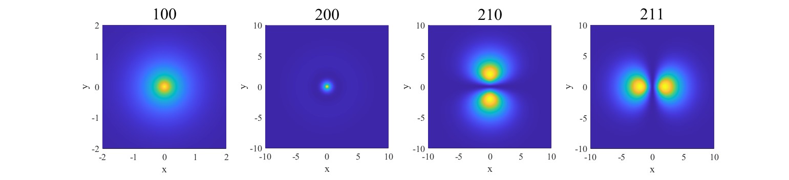
Figure 1. Density plot with\( n = 1 \)and\( n = 2 \).

Images of electron clouds from principal quantum numbers\( n=1 \)to\( n= 2 \)are shown in Figure 1.\( (100) \)or\( 1s \)orbital is the ground state of the hydrogen atom, where the electron has the lowest possible energy. The density plot for this orbital is spherically symmetric, resembling a dense central core that represents a high probability of finding the electron close to the nucleus.\( (200) \)or\( 2s \)is spherically symmetric like the\( (100) \)orbital. Overall, the\( (200) \)orbital is larger than the\( (100) \)orbital, meaning the electron is more spread out.\( (200) \)and\( (210) \)are p orbitals.\( (210) \)is a dumbbell-shaped orbital, aligned along the z-axis, which contains a nodal plane at the\( xy \)-plane, where the electron probability is zero. The regions of highest electron probability are found in two lobes, one above and one below this nodal plane. Similar to\( (210) \),\( (211) \)is also a dumbbell-shaped orbital. The regions of highest electron probability are found in two lobes.

For\( n=3 \)orbitals, the azimuthal quantum number determines the shape of the orbital (spherical for\( s \), dumbbell-shaped for\( p \), and more complex for\( d \)). The magnetic quantum number determines the orientation on the orbital. The density plot is shown in Figure 2.

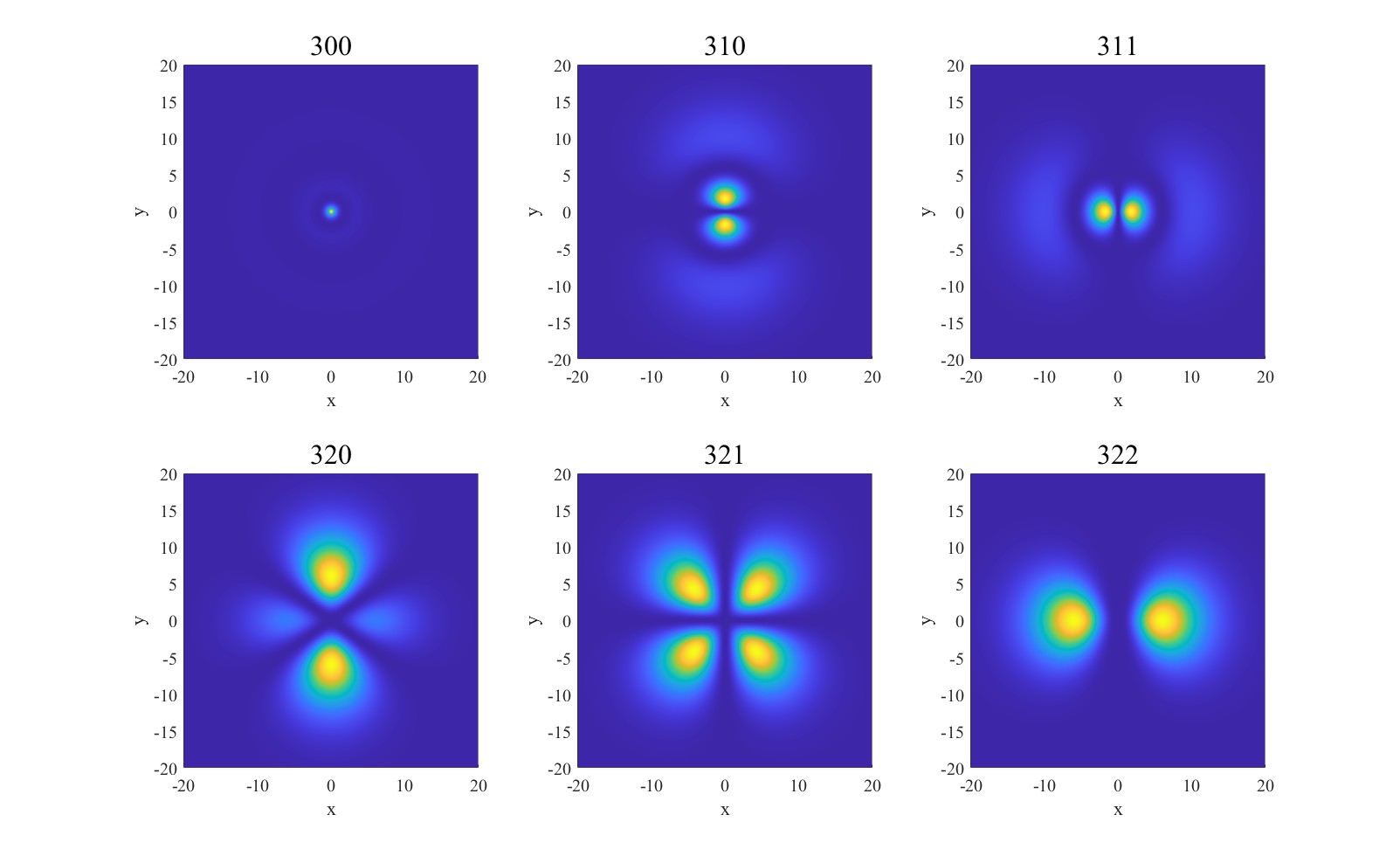
Figure 2. Density plot with\( n=3 \)

2.3.Transition and Spectrum

The energy level of hydrogen atom can be described using Bohr’s model The energy of an electron in nth orbital is

\( {E_{n}}=-\frac{13.6}{{n^{2}}}\ \ \ (19) \)

The hydrogen atom did not stay in one state forever. The state transitions to another state after absorbing energy and releasing energy. The energy level transition formula of hydrogen atom

\( {E_{γ}}={E_{i}}-{E_{f}}=-13.6(\frac{1}{n_{i}^{2}}-\frac{1}{n_{f}^{2}})\ \ \ (20) \)

The transition to a lower state releases energy as a form of light. According to Planck’s formula\( {E_{γ}}=ℏν \), it is possible to get the wavelength of the released photon

\( \frac{1}{λ}=R(\frac{1}{n_{i}^{2}}-\frac{1}{n_{f}^{2}})\ \ \ (21) \)

where\( R \)is the Rydberg constant. Specifically, transitions to\( {n_{f}}=1 \)is called Lymen series, transitions to\( {n_{f}}=2 \)is called Balmer series, and transitions to\( {n_{f}}=3 \)is called Paschen series.

3.Stark Effect

3.1.Basic stark effect

The Stark effect is the shifting and splitting of spectral lines of atoms and molecules due to the presence of an external electric field. The Stark effect can be observed both for emission and absorption lines.

The perturbation theory states that

\( E_{n}^{(1)}=⟨ψ_{n}^{(0)}|{H^{ \prime }}|ψ_{n}^{(0)}⟩\ \ \ (22) \)

The Stark effect originates from the interaction between a charge distribution (atom or molecule) and an external electric field. The interaction energy of a continuous charge distribution\( ρ(\vec{r}) \), confined within a finite volume\( V \), with an external electrostatic potential\( ϕ(\vec{r}) \)is

\( {V_{int}}={H^{ \prime }}=\int _{V}ρ(\vec{r})ϕ(\vec{r}){d^{3}}\vec{r}\ \ \ (23) \)

The first-order\( ϕ(\vec{r}) \)is

\( ϕ(\vec{r})≈ϕ(\vec{0})-\sum _{i=1}^{3}{r_{i}}{F_{i}}.\ \ \ (24) \)

By introducing the electric field

\( {F_{i}}=-{(\frac{∂ϕ}{∂{r_{i}}})|_{\vec{0}}},\ \ \ (25) \)

The interaction terms is

\( {V_{int}}=ϕ(\vec{0})\int _{V}ρ(\vec{r}){d^{3}}\vec{r}-\sum _{i=1}^{3}{F_{i}}\int _{V}ρ(\vec{r}){{r_{i}}d^{3}}\vec{r}=qϕ(\vec{0})-\vec{μ}∙\vec{F}.\ \ \ (26) \)

Thus, the Stark effect is

\( E_{n}^{(1)}=⟨ψ_{n}^{(0)}|{V_{int}}|ψ_{n}^{(0)}⟩=-\vec{F}∙⟨ψ_{n}^{(0)}|\vec{μ}|ψ_{n}^{(0)}⟩.\ \ \ (27) \)

When a hydrogen atom is placed in an external electric field, its spectrum splits. This phenomenon is called the Stark effect.

3.2.Stark Effect of n=2 energy level

Without considering the spin of the electron, the ground state of the hydrogen atom is non-degenerate. The first excited state is quadruple degenerate, and the corresponding wave functions are:\( {ψ_{200}},{ψ_{210}},{ψ_{211}},{ψ_{21-1}} \). The first of these states has zero orbital angular momentum and is called the\( 2s \)state. The last three states have angular momentum of\( l=1 \)and are called\( 2p \)states. They all correspond to one energy eigenvalue

\( E_{2}^{(0)}=-\frac{{e^{2}}}{2a}\cdot \frac{1}{{2^{2}}}.\ \ \ (28) \)

The perturbation Hamiltonian of the electric field is

\( {H^{ \prime }}=-q\vec{E}\cdot \vec{r}=eEz=\frac{{e^{2}}}{a}\frac{z}{a}\frac{eEa}{{e^{2}}/a}=γ\frac{{e^{2}}r}{{a^{2}}}cosθ\ \ \ (29) \)

where\( γ=\frac{eEa}{{e^{2}}/a}≪1 \)is very small.

Next, to find the perturbation matrix\( H \prime \), the author used the equation below [7]

\( cosθY_{m}^{l}(θ,ϕ)=\sqrt[]{\frac{{(l+1)^{2}}-{m^{2}}}{(2l+1)(2l+3)}}Y_{m}^{l+1}(θ,ϕ)+\sqrt[]{\frac{{l^{2}}-{m^{2}}}{(2l-1)(2l+1)}}Y_{m}^{l-1}(θ,ϕ)\ \ \ (30) \)

Therefore,

\( ⟨{ψ_{200}}|{H^{ \prime }}|{ψ_{200}}⟩=⟨{ψ_{210}}|{H^{ \prime }}|{ψ_{210}}⟩=⟨{ψ_{211}}|{H^{ \prime }}|{ψ_{211}}⟩=⟨{ψ_{21-1}}|{H^{ \prime }}|{ψ_{21-1}}⟩=0\ \ \ (31) \)

\( ⟨{ψ_{200}}|{H^{ \prime }}|{ψ_{21±1}}⟩=⟨{ψ_{210}}|{H^{ \prime }}|{ψ_{21±1}}⟩=⟨{ψ_{211}}|{H^{ \prime }}|{ψ_{21-1}}⟩=0\ \ \ (32) \)

The nonzero matrix element is

\( ⟨{ψ_{200}}|{H^{ \prime }}|{ψ_{210}}⟩=⟨{ψ_{210}}|{H^{ \prime }}|{ψ_{200}}⟩=-3\frac{{e^{2}}}{a}\ \ \ (33) \)

The perturbation matrix\( {H^{ \prime }} \)is

\( {H^{ \prime }}=[\begin{matrix}0 & -3\frac{{e^{2}}}{a} & 0 & 0 \\ -3\frac{{e^{2}}}{a} & 0 & 0 & 0 \\ 0 & 0 & 0 & 0 \\ 0 & 0 & 0 & 0 \\ \end{matrix}],\ \ \ (34) \)

and the eigenvalue of this matrix is

\( E_{2,1}^{(1)}=3\frac{{e^{2}}}{a}γ,E_{2,2}^{(1)}=-3\frac{{e^{2}}}{a}γ,E_{2,3}^{(1)}=0,E_{2,4}^{(1)}=0.\ \ \ (35) \)

Thus, the degenerated state is split into three spectra. One is

\( E_{2}^{(0)}+E_{2,1}^{(1)}=-\frac{1}{{2^{2}}}\frac{{e^{2}}}{a}+3\frac{{e^{2}}}{a}γ=-\frac{1}{4}\frac{{e^{2}}}{a}+3eEa\ \ \ (36) \)

The corresponding wave function is given by

\( ψ_{1}^{(0)}=\frac{1}{\sqrt[]{2}}({ψ_{200}}-{ψ_{210}})\ \ \ (37) \)

Similarly, the energy and wave function of another state are

\( E_{2}^{(0)}+E_{2,2}^{(1)}=-\frac{1}{{2^{2}}}\frac{{e^{2}}}{a}-3\frac{{e^{2}}}{a}γ=-\frac{1}{4}\frac{{e^{2}}}{a}-3eEa\ \ \ (38) \)

\( ψ_{2}^{(0)}=\frac{1}{\sqrt[]{2}}({ψ_{200}}+{ψ_{210}})\ \ \ (39) \)

So,\( n=2 \)energy level is split into 3 new energy levels. According to theory, the energy level of degree\( {n^{2}} \)degeneracy will be symmetrically split into\( N=2n-1 \)energy levels [7]. This result is completely consistent with the theory.

3.3.Stark effect in higher energy levels

Despite using the wave function, the perturbation Hamiltonian matrix is also can be used to obtain the Stark effect. The nonzero Hamiltonian matrix element can be calculated by [8]

\( H{ \prime _{l,l+1}}=-\frac{neϵ{a_{0}}}{2}{\frac{(n-l-1)!}{2n{[(n+l)]^{3}}}^{1/2}}\cdot {\frac{(n-l-2)!}{2n{[(n+l+1)]^{3}}}^{1/2}}(n+1)!(n+l+1)!(2l+5)\sum _{k}(\frac{3}{n-l-1-k})(\frac{1}{n-l-2-k})(\frac{2l+4+k}{k})\cdot \sqrt[]{\frac{{(l+1)^{2}}-{m^{2}}}{(2l+1)(2l+3)}} (40) \)

This method can examine the Stark effect energy level correction at n=3, n=4 and n=5 energy levels [9]. Just as the author did with the electron cloud before. Also, it is possible to use software to simulate the Stark effect. Mathematica can calculate the matrix element and the correction wavefunction, which can significantly reduce manual work [10].

4.Conclusion

Starting from the basic quantum mechanics principles of hydrogen atoms, this article deduces the Schrödinger equation of hydrogen atoms, and also discusses its solution and its importance to the development of quantum mechanics. The successful derivation of this equation laid a solid foundation for subsequent research. Then, using modern computational tools, this paper show how abstract quantum mechanical formulas can be transformed into intuitive descriptions of the hydrogen atom’s electron cloud. The author uses computational simulations to reveal the density distribution of electron clouds and the probability distribution of electrons at different energy levels. These simulations not only help us visually understand the internal structure of atoms, but also provide a visual tool for further studying the properties of hydrogen atoms. Afterwards, the article discusses in depth the emission and absorption spectral lines of hydrogen atoms, which provide valuable clues for exploring more complex atomic and molecular systems. The focus of the article focuses on the Stark effect of hydrogen atoms at the n=2 energy level. The article not only shows how to use the perturbation Hamiltonian matrix formula to accurately calculate the high-energy Stark effect, but also shows that it is completely feasible to programmatically calculate the Stark effect at higher energy levels. Through these calculations, people were able to reveal how external electric fields affect the splitting and energy changes of hydrogen atoms’ energy levels, which is crucial for understanding the microscopic mechanisms of how atoms respond to electric fields.

References

[1]. Griffiths, David J., Schroeter, Darrell F. Introduction to Quantum Mechanics (3rd Ed). Cambridge University Press.
[2]. Zeng, Jinyan. (2022). Quantum Mechanics, volume I (5th Ed.). Science Press.
[3]. Hicks, William W (1973). High-frequency stark effect and its application to plasma diagnostics. United States.
[4]. Wright, D., Sangtarash, S., Mueller, N. S., Lin, Q., Sadeghi, H., & Baumberg, J. J. (2022). Vibrational Stark Effects: Ionic Influence on Local Fields. Journal of Physical Chemistry Letters, 13(22), 4905–4911.
[5]. Robyr, J.-L., Knowles, P., & Weis, A. (2010). Stark shift of the Cs clock transition frequency: a new experimental approach. IEEE Transactions on Ultrasonics, Ferroelectrics, and Frequency Control, 57(3), 613–617.
[6]. Su, Yanfei., Zhang, Changxin., Xi, Wei. (2004). Energy level splitting of the Hydrogen atom in Stark’s effect. College Physics, 23(2), 8-10.
[7]. Zheng, Lixian. (2003). The popular formula of perturbative matrix elements of the Stark effect of the hydrogen atom. College Physics, 22(1), 41-42.
[8]. Zhang, Changxin., Xi, Wei., Su Yanfei. (2004). A formula of energy level for hydrogen atom in Stark effect. College Physics, 23(12), 21-24.
[9]. Xu, Jianliang., Tang, Bingshu. (2005). Numerical Calculation of Stark Effect in Hydrogen Atom. Journal of Anqing Teachers College (Natural Science), 11(2), 23-26.
[10]. Fontanari, D., Sadovskií, D. A. (2015). Perturbations of the hydrogen atom by inhomogeneous static electric and Magnetic Fields. Journal of Physics A: Mathematical and Theoretical, 48(9), 095203.
Cite this article
Ren,B. (2024). Exploring the hydrogen atom: From wave function to stark effect. Theoretical and Natural Science,30,187-194.
Data availability
The datasets used and/or analyzed during the current study will be available from the authors upon reasonable request.
Disclaimer/Publisher's Note
The statements, opinions and data contained in all publications are solely those of the individual author(s) and contributor(s) and not of EWA Publishing and/or the editor(s). EWA Publishing and/or the editor(s) disclaim responsibility for any injury to people or property resulting from any ideas, methods, instructions or products referred to in the content.
About volume
Volume title: Proceedings of the 3rd International Conference on Computing Innovation and Applied Physics
© 2024 by the author(s). Licensee EWA Publishing, Oxford, UK. This article is an open access article distributed under the terms and
conditions of the Creative Commons Attribution (CC BY) license. Authors who
publish this series agree to the following terms:
1. Authors retain copyright and grant the series right of first publication with the work simultaneously licensed under a Creative Commons
Attribution License that allows others to share the work with an acknowledgment of the work's authorship and initial publication in this
series.
2. Authors are able to enter into separate, additional contractual arrangements for the non-exclusive distribution of the series's published
version of the work (e.g., post it to an institutional repository or publish it in a book), with an acknowledgment of its initial
publication in this series.
3. Authors are permitted and encouraged to post their work online (e.g., in institutional repositories or on their website) prior to and
during the submission process, as it can lead to productive exchanges, as well as earlier and greater citation of published work (See
Open access policy for details).