


1. Introduction
Appreciating music is a breeze for most people, but for the hearing impaired, it is a huge challenge. However, with the visual representation of music, we can transform music into a visual piece to compensate for their auditory deficiencies, allowing them to be more engaged in experiencing music and even experimenting with instrumental learning.
In recent years, there has been a proliferation of music visualization methods as data visualization techniques have advanced. However, most of the methods rely on the color saturation, transparency, size of the graphs and their variations to show changes in pitch and volume. Most of these are artistic re-creations, and the presentation is often abstract and irregular, requiring viewers to rely on their personal feelings for interpretation. These methods have not yet accurately quantified the basic characteristics of music and therefore fail to accurately assist the hearing impaired in learning music or musical instruments.
Chladni Patterns [1] is a promising solution. The basic idea is that when the intrinsic frequency of a thin plate is matched to an external vibration source, the plate produces specific ripple patterns. By placing particles on the plate, these vibration patterns are significantly enhanced at specific locations, and the particles move along the ripple lines to form unique patterns [2] . This opens the door to combining the acoustic properties of music with visual patterns, providing a more intuitive musical experience for the hearing impaired.
Past research has explored several aspects of the Chladni pattern. For example, Worlan [3] used it to help students understand standing wave phenomena in acoustics; Li-Chan Lin [4] et al. developed a plug-in multifunctional resonance and standing wave demonstration device, which is capable of visualizing a wide range of vibration phenomena such as chords, circles, free-end reflections, Lissauer graphs, and Chladni patterns, which can help students to better understand vibration and resonance phenomena. Hu Jing [5] et al. improved the experimental method by adding Bluetooth connectivity to mobile phones and adopting Phyphox software and piano software in smartphones as sound sources to improve the traditional Chladni plate experiment, while Coughlin [6] delved into the creation of Chladni patterns. However, although studies have focused on the use of particles to form Chladni patterns, there have been few systematic studies on the factors affecting Chladni patterns.
In terms of combining music and interactive images, Beane [7] explores multimedia performances of music with interactive images, while Li [8] focuses on real-time music visualization in relation to Chladni patterns. However, most of these studies do not fully integrate the physical properties of Chladni patterns with music visualization.
Amin’s [9] research aims to establish theoretical formulas to create a unique space that combines elements of music and architecture through the study of Chladni patterns. However, this article does not seem to relate the theoretical formulas to the physical properties of the lamellas.
Taken together, the current research on how particles form Chladni patterns has not yet fully explored in depth the various factors that influence their generation, which includes particle characteristics, plate properties, and parameters of the vibration source. This means that further research is still needed to deepen our understanding of the effects of these factors on the morphology of Chladni patterns. In addition, while there are studies that have explored the fundamentals of Chladni patterns, there is a lack of research related to how to accurately map specific musical compositions onto Chladni patterns. This requires a close integration of the acoustic properties of music with the process of Chladni pattern formation.
In this study, we delve into the use of the finite element method to visualize and compare Chladni patterns with piano tones. It is structured as follows. Firstly, we present the complete list of modes for a flat plate using finite element modal analysis, with the intention of exploring whether the structure of the modal analysis can be fully demonstrated the Chladni pattern for musical tones, and experimental modal analysis was used to validate the accuracy of the finite element model. Secondly, we explore how Chladni patterns can be used to present real musical fragments. Finally, the overall study is summarized and future research directions are envisioned.
2. Finite Element Modal Analysis of Simulated Cranial Graphs Finite Element Analysis of Circular Plate Cranial Graphs
2.1. FEA analysis - parameter identification, mesh convergency study, results
In order to accurately identify all the vibration modes that can be excited within the frequency range of the piano keys, we chose to utilize the finite element analysis tool, ANSYS, for modal analysis. Within the software, we set the material properties and boundary conditions of the plate. With these settings, we successfully calculated all the vibration modes and their corresponding intrinsic frequencies for the specified frequency range.
We chose an acrylic circular plate with a diameter of 250 mm, a thickness of 0.8 mm and a central circular hole aperture of 6.2 mm as the geometric model for the FEA. This plate has the largest diameter and the thinnest thickness in our experiments, and is theoretically more likely to excite larger amplitudes.
It is very important to select and set the appropriate parameters before performing finite element analysis for specific vibration modes. The following is the setup and the associated material determination process that we performed for this study.
The hammering method based on GB/T 22315-2008 [10] national standard provides us with a method to determine Young’s modulus. With this method, we can ensure that our simulations are closer to the actual physical properties.
It is crucial to ensure accurate material parameters before performing finite element analyses. We have adopted the national standard hammering method to estimate the material properties of acrylic sheets, focusing mainly on the determination of Young’s modulus. The principle of the hammering method is based on the Fourier theory, which states that any periodic function can be viewed as a superposition of sinusoids of different amplitudes and phases. In a certain frequency range, the hammering impulse can be regarded as consisting of an infinite number of sinusoids with similar amplitudes, so that all resonance peaks in the frequency range will be excited. By identifying the frequency of the first resonance peak and applying the relevant theoretical equations, we can invert the Young’s modulus of the material.
We used an acrylic beam with dimensions of 180mm x 10mm x 3mm as our test material, whose mass was determined to be 5.3g, leading to a deduced density of 982kg/m3 . We chose to fix a section of the acrylic beam to the experimental table by means of iron clips and attach a piezoelectric accelerometer CT1000L to the top of the beam, which allowed us to measure its vibration response and thus obtain information about its natural frequency and vibration pattern. By evaluating the natural frequency of the beam, it was then used to derive the Young’s modulus.
During the measurements, we considered the clamping of the beam and determined the effective beam length to be 145 mm. Figure 1.(a) and (b) show the front and side views of the experimental setup, respectively.
|
|
(a) Front view | (b) Side view |
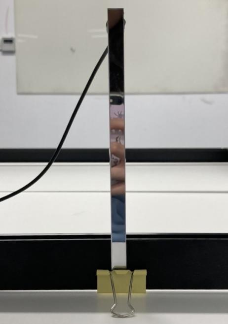
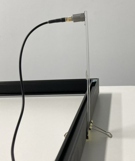
Figure 1. a, b Front and side views of the hammering experimental setup
The acceleration sensor and the dynamic force transducer CT-LC-01 impact hammer are connected to a signal conditioner and to a computer via the MCC USB-1608G digital-to-analogue converter card. The digital signals are finally recorded and analysed.
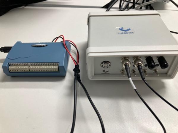
Figure 2. Data processing apparatus used for hammering experiments
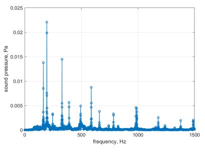
As shown in Figure 3, we observe the spectrum of the acceleration response of the free end of the beam and from it we clearly derive the first order natural frequency as 7.98 Hz.
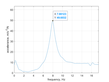
Figure 3. Free end acceleration spectrum of beams
It is worth emphasizing that the theoretical formulae of the national standards are not fully applicable in this experiment. There are two main reasons for this: firstly, the mass of the accelerometer used is as high as 8.7 g, which is significantly greater than the mass of the beam, and this is not taken into account in the theoretical formula. Secondly, the two key physical properties of acrylic, Young’s modulus and Poisson’s ratio, remain unknown. To address these issues, we turned to the numerical simulation technique of Ansys and determined the most suitable acrylic material parameters through parameter optimization.
For the finite element modelling, we considered the sensor as a point mass and placed it at 11.6 mm from the free end of the beam. The beam was modelled as a 2D shell unit using FEA software. The initial Young’s modulus and Poisson’s ratio were obtained based on a web search with values of 3 GPa and 0.37, respectively. The simulation results show that the intrinsic frequency of the first bending mode is 14.729 Hz (see Figure 4 for details). This frequency is almost twice the experimentally measured frequency.
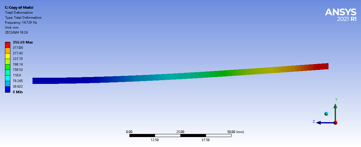
Figure 4. Finite element modal analysis results (initial elastic properties)
After careful iterative optimisation, we determined the Young’s modulus of the acrylic sheet to be 0.880 GPa, as well as the Poisson’s ratio to be 0.402. Equipped with these precise material parameters, we further carried out a finite element modal analysis of the disc.
The size of the grid cells is a key parameter during finite element simulation. Choosing a smaller cell size results in a solution that is closer to the real one, but this also leads to an increase in computation time. Therefore, a trade-off must be reached between cell size and computational accuracy. By performing a mesh convergence analysis, we can determine if this trade-off has been found. For our disc model, we tried three different cell sizes: 27mm, 5mm and 1mm.
Table 1. Grid Convergence Study
Unit size | 27 mm | 5 mm | 1 mm |
First modality | 130 Hz | 130 Hz | 130 Hz |
Second modality | 141 Hz | 141 Hz | 140 Hz |
Third Modality | 221 Hz | 220 Hz | 220 Hz |
(in the frequency range) The last modality | 597 Hz
| 575 Hz
| 575 Hz
|
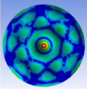 Figure 1
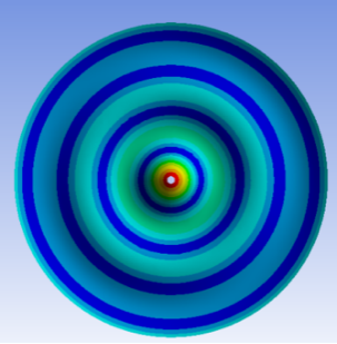 Figure 2
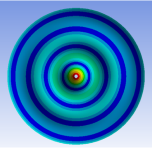 Figure 3
As can be seen from Table 1, by comparing the modal natural frequencies at different cell sizes, it is possible to determine whether the mesh has converged or not. When the mesh is refined to 5mm or 1mm, the mesh has reached convergence and no further refinement is needed. Therefore, in the next simulation, we use 2mm as the cell size of the mesh.
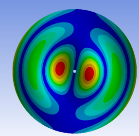
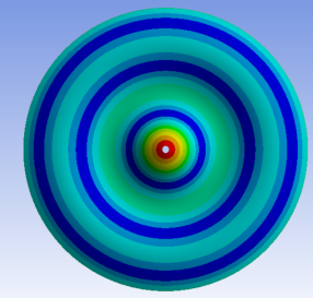
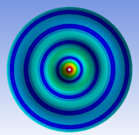
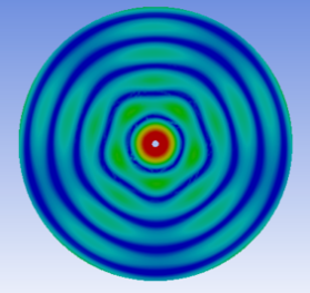
Some of the ANSYS simulation results for the selected size of acrylic circular plate are shown in Table 2.
Table 2. ANSYS Partial Simulation Results with Corresponding Frequencies (Hz)
|
|
|
219.5 | 321 | 575 |
2.2. Hammer test validation of finite element modal analysis
To further verify this and validate the accuracy of the finite element model, we will use the hammering method to perform a modal analysis on the acrylic circular plate used in the particle experiments. With this method, we expect to obtain the Chladni pattern of the circular plate itself and compare it with the results of the finite element analysis.
In a hammering experiment, we can use the following equation to represent the frequency response function of the system:
\( \frac{d}{F}=\frac{{φ_{in}}{φ_{out}}}{-m{ω^{2}}+k+cjω}\ \ \ (1) \)
In this equation, d represents the spectrum of the displacement, F represents the spectrum of the force, the \( {φ_{in}} \) and \( {φ_{out}} \) represent the modal vectors at the excitation and response points, respectively. Also, m, k and c represent the modal mass, stiffness and damping coefficients, respectively.
This equation reveals the close relationship between the frequency response function and the position of the knock and the vibration acquisition position. By tapping at two different positions and keeping the vibration acquisition position constant, we can obtain two different frequency response functions. Calculating the ratio of these two frequency response functions gives us the relative amplitudes of the plate at different positions. These relative amplitudes present us with the vibration modes of the plate, which is often referred to as the Chladni pattern.
2.3. Experimental design
As shown in Figure 5, we used four fishing lines and strong rigid springs to suspend the ends of the sheet on a sturdy frame on either side and keep them parallel to the ground.
In order to obtain comprehensive information on the modal shapes, we chose to perform tapping at different locations, placing the accelerometer in the centre of the sheet. Given that most of the modes are symmetrically distributed, a modal analysis experiment on only one quarter of the plate is sufficient to obtain modal information for the whole plate. We divided the quarter sector of the circular plate into three equal parts, and set five tapping points uniformly along the radius of each part, for a total of 13 tapping points.
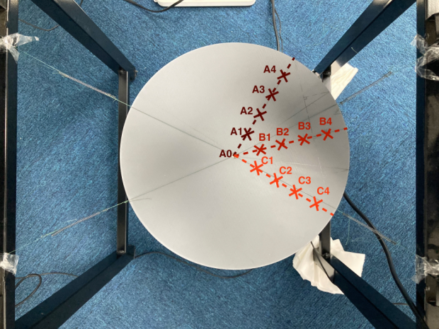
Figure 5. Knock positions for experimental modal analysis
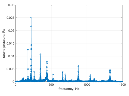
The same data acquisition equipment and modal analysis methods were used in order to investigate the vibration characteristics of the acrylic sheet. By performing 20 to 30 taps at each point and calculating the ensemble average of the frequencies, the effect from double-tap tapping can be reduced to some extent. Finally, we combine the amplitude data obtained at each time and calculate the average value, and the typical acceleration frequency response function is shown in Figure 6.
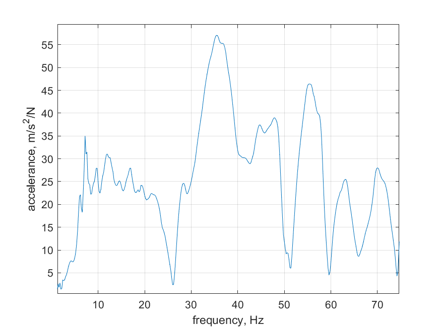
Figure 6. Frequency Response Function at the centre of the circle A0 point
2.4. Results of the hammer test
By averaging the frequency response function over the data from the 13 tapping points, we have successfully derived the first four modes of the structure and the results are shown in Figure 7.
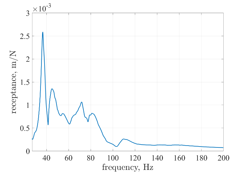
Figure 7. Average displacement frequency response function for 13 points
We observed that in the first mode of the experiment, the frequency was 36.7 Hz. Subsequently, by comparing the ratios of the imaginary part of the resonance peak in the frequency response function at different tapping points, we were able to infer the displacement and phase of the different points on the circular plate at that frequency. In order to present this data more visually, we show this information in three dimensions in Figure 7.
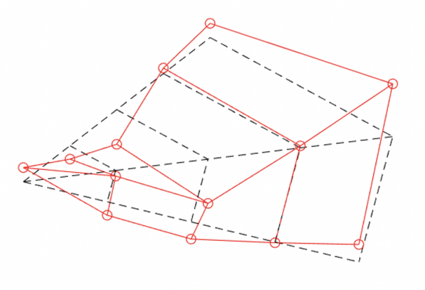
Figure 8. 3D modes of experimental results
In order to compare more conveniently with the modal diagrams of FEA (Figure. 9), we transformed the 3D modal diagrams into 2D images (Figure. 10) to show the vibration of the modes at 0 degree, 45 degree and 90 degree. By comparing these two images, it can be clearly observed that the simulation results of the finite element analysis are highly consistent with the results of the tapping experiments, especially in the radius direction, both of which show a downward concave curve.
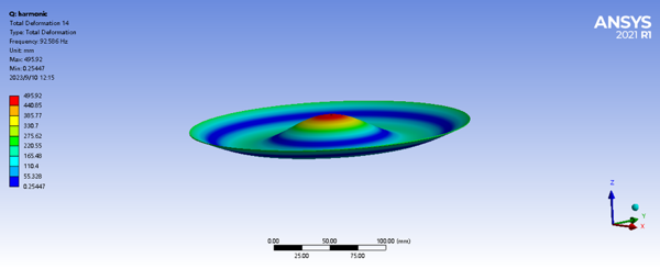
Figure 9. Finite element modes corresponding to experimental modes

Figure 10. Mode shapes in the radius direction
However, despite the similarity of the modes, we note that the resonance frequency of the FEA is approximately about three times the experimental modal frequency. After revisiting the differences between the FEA setup and the experiments, we found that two factors were not taken into account in the simulations: the mass of the accelerometer used in the experiments and the stiffness of the spring used to suspend the circular plate in the experiments.
After the accelerometer only and the spring mass are taken into account in the finite element model, the updated simulation results are shown in Table 3, from I we can see that the frequencies of the finite element simulation are highly consistent with the frequencies of the experimental modes.
Table 3. Comparison of frequencies obtained from experiment and simulation (addition of accelerometer mass and virtual spring)
Experimentally obtained frequencies (Hz) | Frequency obtained by simulation (Hz) |
36.7 | 37.74 |
45.1 | 48.83 |
71.8 | 70.31 |
81.1 | 84.01 |
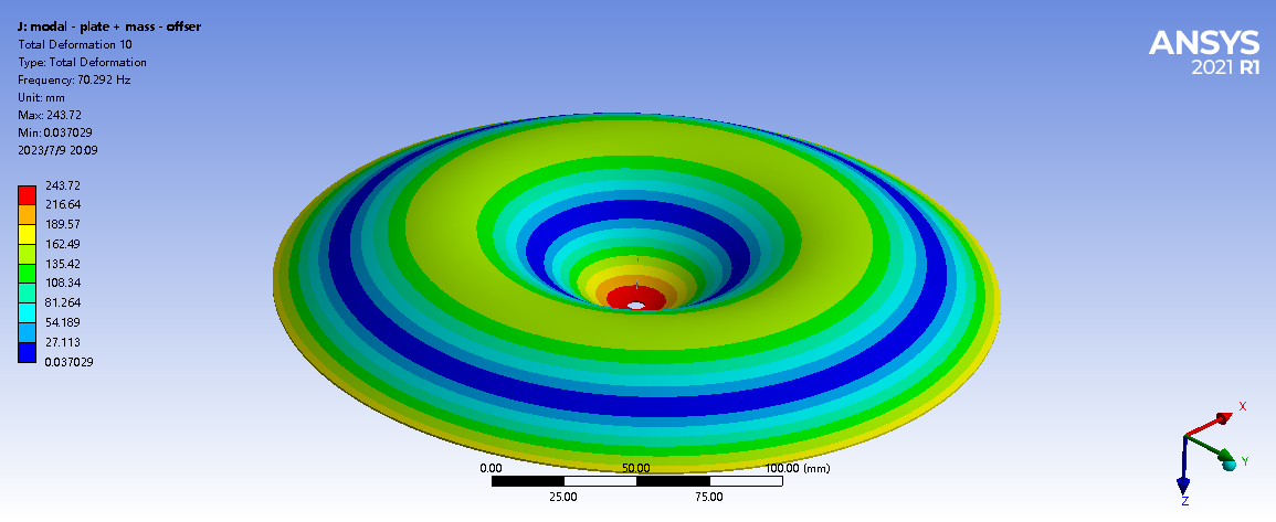
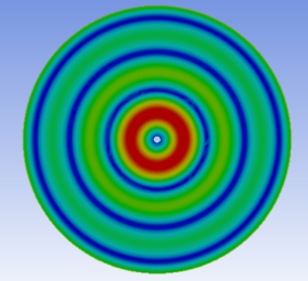
Figure 11. Chladni pattern of a circular plate with centre point mass and virtual spring added
After comprehensively considering all the factors affecting the resonance frequency and modes in the experiment, we successfully obtained a Chladni pattern simulation that is highly consistent with the experimental results. This means that in subsequent studies, we can eliminate the tedious experimental steps and directly use finite element analysis tools such as ANSYS to accurately simulate the Chladni patterns, so as to study the relationship between the Chladni patterns and music more effectively.
3. Using Chladni pattern to visualize a piano melody
We performed a harmonic analysis using Finite Element Analysis software and indeed verified that a single plate excites modes corresponding to all the piano keys. Based on this finding, we further intend to relate the frequencies of the piano keys to the Chladni pattern. Therefore, the goal of this chapter is to delve into the study of Chladni patterns in analogue piano melodies.
A piano melody consists of single notes of different pitches and their harmonies. Several key musical elements, such as pitch, volume and note timings, play a central role in performance. In order to effectively simulate the clavier figure of a piano melody, we decided to start with the most basic single notes and explore how these musical elements affect the sound properties of the piano.
In the previous section, we started from the point of view of monophonic properties, and investigated the different voicing characteristics that monophonic tones may exhibit under different conditions of pitch, intensity and note duration. This lays the foundation for this part of the study, in which we will further explore the acoustic properties of choruses as well as more complex melodies.
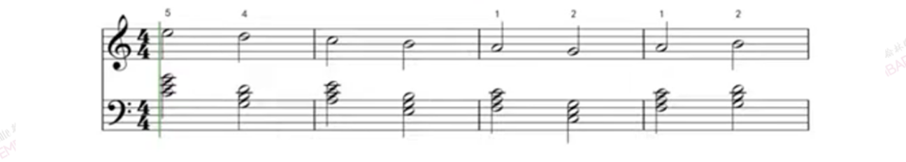
Figure 12. Canon (excerpt) piano pentatonic score
We chose the melody Canon due to its simple melodic structure in order to investigate the feasibility of Chladni patterns in clearly expressing a melody. In order to obtain the magnitude of the sound pressure at different frequencies, we used the short-time Fourier transform method to analyse the recorded audio of a 200-second excerpt of the Canon melody. The short-time Fourier transform splits the audio into 1-second segments and applies the Fourier transform to each 1-second segment. In order to maintain the continuity of the color map and reduce horizontal interference, the analysis of each segment included a 0.5 second overlap. Ultimately, the results of the analysis of all the segments form the color map in Figure 13.
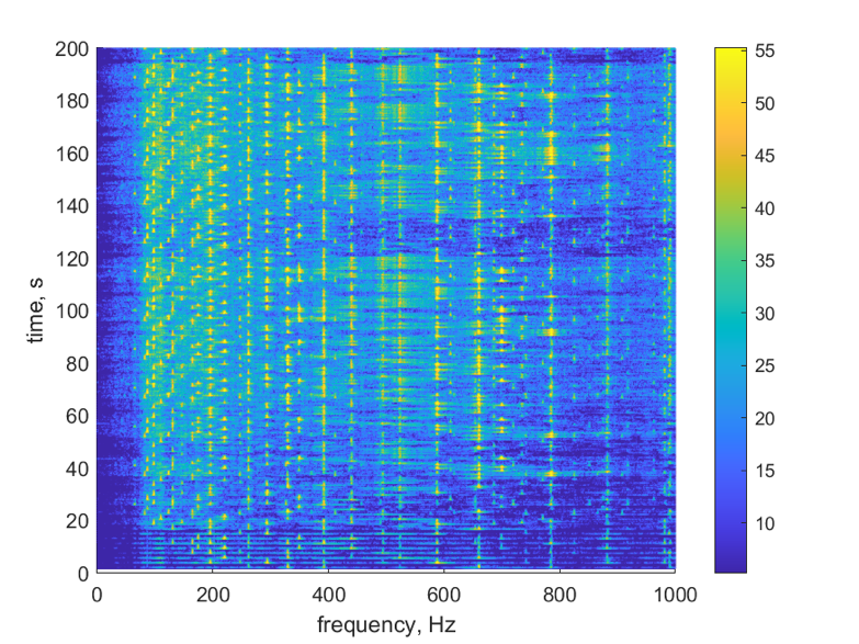
Figure 13. Colour map of the short-time Fourier transform of the Canon (excerpt) recording
From Figure 13 we can observe that each note has a distinct fundamental frequency component. However, it is difficult to clearly identify the main notes at different points in time in this plot, and therefore it is impossible to match them to the score. In addition, the colour representation in the plot is not intuitive and it is difficult to accurately reflect the difference in magnitude of the amplitudes.
Therefore, in order to present a clearer picture of the different combinations of pitches that make up a melody, we try to introduce a Chladni pattern. This will help to visualise the dominance of the different notes in a more intuitive way and provide more accurate information about the amplitude.
In order to accurately match the graphs to the specific piano keys on the score, we need to determine the fundamental frequency corresponding to each waveform. Therefore, we converted the audio recording to a time domain signal to clearly observe the chorus waveforms generated by each key press. This step will help to accurately identify the fundamental frequency of each note that corresponds to a specific piano key.
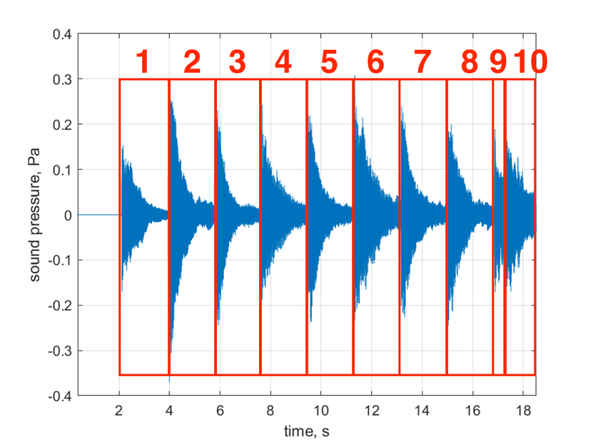
Figure 14. Plot of time-domain data for the Canon (excerpt) recording
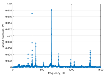
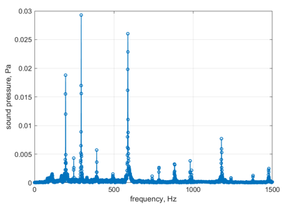
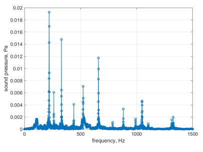
Subsequently, we did the Fourier transform for each combination of tones and summarised the corresponding fundamental frequency and maximum sound pressure for each combination of tones through Table 4.
Table 4. Fourier transform results for 5 combinations of tones with corresponding fundamental frequency and maximum sound pressure
Time (s) | Sequence of the combination of tones | Results of Fourier transform | Fundamental frequencies (Hz) | Maximum sound pressure (Pa) |
2.0673 | / | / | / | / |
3.89859 | 1 |
| 660 | 0.018 |
5.78565 | 2 |
| 294 | 0.029 |
7.6085 | 3 |
| 220 | 0.019 |
9.41683 | 4 |
| 195 | 0.022 |
11.2916 | 5 |
| 220 | 0.025 |
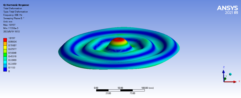
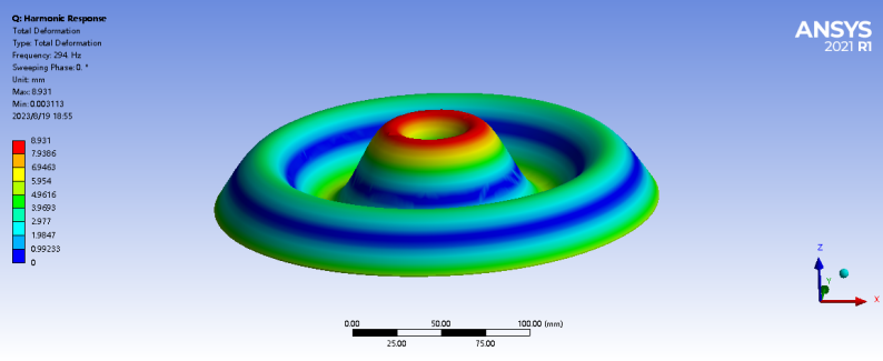
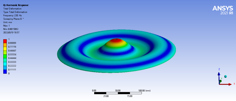
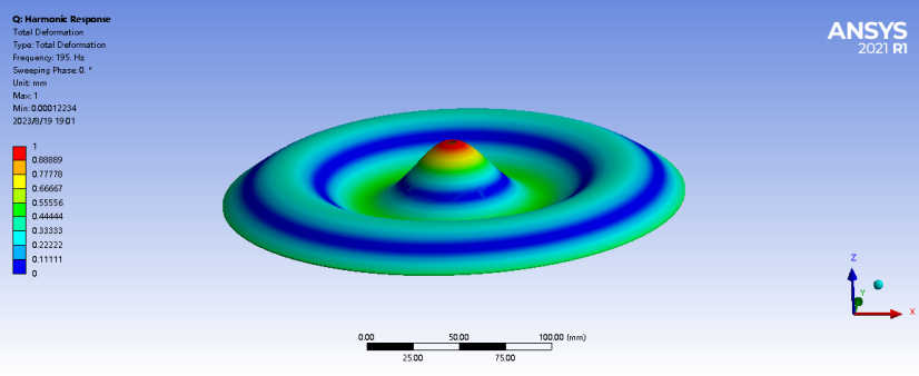
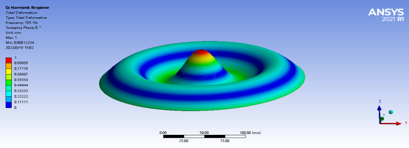
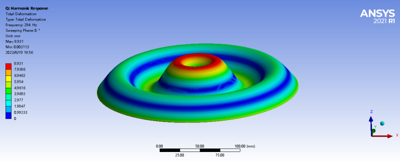
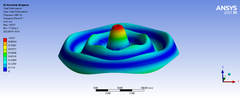
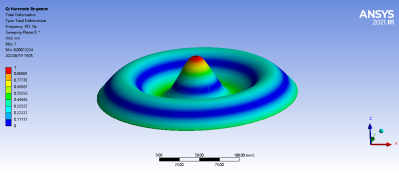
After obtaining the frequency values, we can use the harmonic response function in FEA to simulate the corresponding Chladni patterns to reflect the different fundamental frequencies. The results of these simulations are shown in Table 5.
Table 5. Graphical simulation of harmonic response Chladni
Sequence of combination of tones | Fundamental frequencies (Hz) | Maximum amplitudes (V) | Corresponding Chladni pattern |
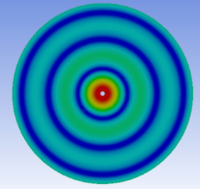
1 | 660 | 0.18354 |
|
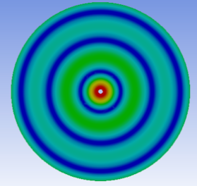
2 | 294 | 2.59 |
|
3 | 220 | 0.19 |
|
4 | 195 | 0.22 |
|
5 | 220 | 0.25 |
|

Although we have succeeded in transforming the abstract Fourier transform results into Chladnian graphs with distinct shapes through the correspondence between fundamental frequency and maximum magnitude, it is still difficult to visually compare the difference in magnitude of the maximum magnitude due to its relatively small value.
Therefore, the following steps were planned to highlight the differences between the different amplitudes in order to present more clearly and visually the different volume and intensity variations of the different notes as they are played (see Table 6):
1. The vibrational shape of the Chladni graph was obtained from the harmonic response data used in the previous table.
2. Standardise the maximum amplitude to 100 mm.
3. These amplitudes are amplified according to the maximum sound pressure at a particular frequency.
This series of steps will help to compare the differences in volume and intensity of different notes in a clearer and more visual way.
Table 6. Chladni patterns with amplified amplitudes
Sequence of combination of tones | Fundamental frequencies (Hz) | Corresponding Chladni patterns |
1 | 660 |
|
2 | 294 |
|
3 | 220 |
|
4 | 195 |
|
5 | 220 |
|
6 | 195 |
|
7 | 220 |
|
8 | 293 |
|
9 | 660 |
|
10 | 196 |
|
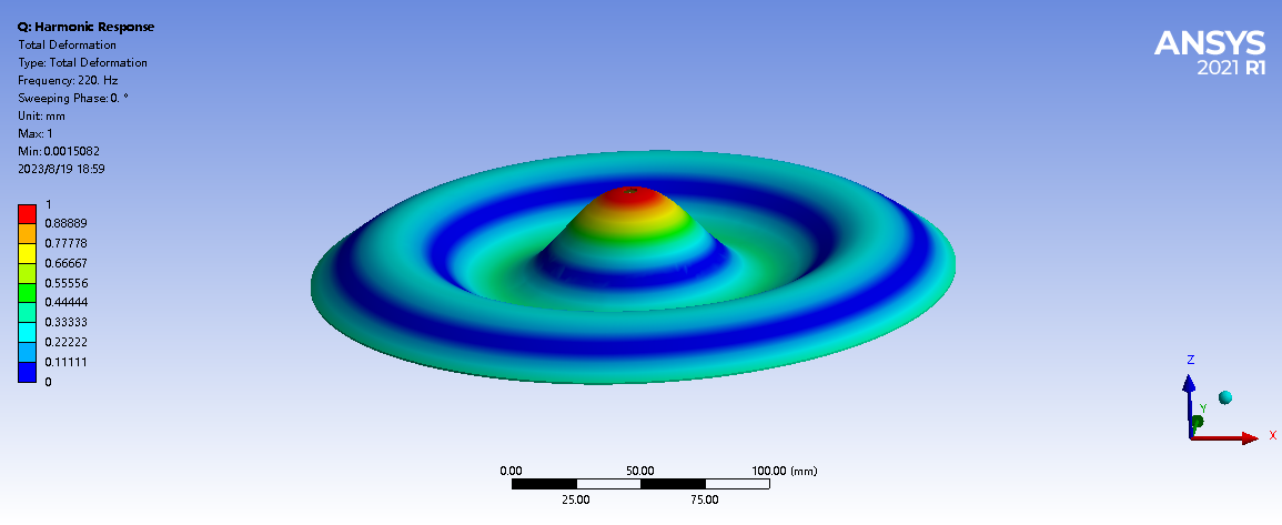

In the music visualisation study in this chapter, we have chosen the single tone that has the highest pitch in a very short time period and used this single tone to pick the corresponding Chladni pattern for the simulation visualisation.
4. Conclusion
The main goal of this research is to study in depth the relationship between Chladni patterns and music and to find a visualisation method to present the characteristics of music in a visual form. In order to achieve this goal, a series of numerical simulations have been carried out in order to study in detail the mechanism of Chladni pattern generation and to analyse the influence of factors such as frequency and board specifications on Chladni patterns.
We first observed that the distribution of particles on the plate is very complex, especially when the frequency lies between two neighbouring natural frequencies. Through numerical simulations, we successfully solved this problem. At the same time, we recognise that there is a certain complexity in vibration modal analysis that requires further in-depth study.
In order to establish the relationship between the Chladni pattern and the piano key frequency, we used several finite element simulation methods. Firstly, we used ANSYS to perform modal analysis simulations covering all excitable modes in the pianoforte frequency range. However, since the natural frequencies of the simulation results are slightly different from those of the actual granular experiment, we used the hammering method to verify the simulation results. We demonstrated that finite element modal analysis can simulate the dynamic properties of the circular plate well, and found that different excitation frequencies may also have some effects on the Chladni pattern in a smaller frequency range. This means that a plate with a specific shape and size can effectively reflect the full range of key sounds of a piano, overcoming the previous problem of needing multiple plates of different shapes and sizes to visualise most of the piano keys.
In order to further simulate elements in the music, we have not only visualised single tone frequencies, but also successfully visualised a piece of music using finite element harmonic analysis methods.
However, this study also revealed some obvious limitations. In order to realise the full potential of Chladni graphs, future research could be carried out in the following areas:
• More in-depth vibration modal analysis: further study of the complexity of vibration modes, especially in the case of frequency-adjacent regions, to improve the accuracy of simulation results.
• Optimisation of the simulation methodology: the simulation methodology was improved in order to solve the problems of high similarity of some graphs and the blurring of the bourdon lines and to make the Chladni patterns more suitable for music education and analysis.
References
[1]. Chladni E F F. Die akustik [M]. Breitkopf & Härtel, 1830.
[2]. Gough C. The violin: Chladni patterns, plates, shells and sounds [J]. The European Physical Journal Special Topics, 2007, 145(1): 77-101.
[3]. Rossing T D. Teaching physics of music [J]. Bulletin of the American Physical Society, 2009, 54.
[4]. Li-Chan Lin, Jin-Fen Lin, De-An Li. Multifunctional resonance-standing wave demonstrator [J]. Physics Teaching, 2016 (4): 27-29.
[5]. J. Hu, S. Zhou, X. Li, et al. Exploring the improvement of the Chladni plate for sound visualization [J]. University Physics Experiment, 2022, 35(6): 55-58.
[6]. Coughlin A M. Patterns in the sand: Mathematical exploration of Chladni patterns [J]. Journal of Mathematics and Science: Collaborative Explorations, 2000, 3(1): 131-146.
[7]. A B. Generating audio-responsive video images in real-time for a live symphony performance [D]. Texas A&M University, 2007.
[8]. Li L. Research and implementation of real time music visualization [C]//Second International Symposium on Computer Technology and Information Science (ISCTIS 2022). SPIE, 2022, 12474: 594-600.
[9]. Amin, P. “Music As a Tool For Ecstatic Space Design.” (2023).
[10]. National Steel Standardization Technical Committee. Test Methods for Modulus of Elasticity and Poisson’s Ratio of Metallic Materials: GB/T 22315 - 52008 [S]. Beijing: China Standard Press, 2008.
Cite this article
Xia,Y. (2024). Seeing the piano sound -- Exploration on utilizing finite element analysis to visualize piano sound. Theoretical and Natural Science,30,216-231.
Data availability
The datasets used and/or analyzed during the current study will be available from the authors upon reasonable request.
Disclaimer/Publisher's Note
The statements, opinions and data contained in all publications are solely those of the individual author(s) and contributor(s) and not of EWA Publishing and/or the editor(s). EWA Publishing and/or the editor(s) disclaim responsibility for any injury to people or property resulting from any ideas, methods, instructions or products referred to in the content.
About volume
Volume title: Proceedings of the 3rd International Conference on Computing Innovation and Applied Physics
© 2024 by the author(s). Licensee EWA Publishing, Oxford, UK. This article is an open access article distributed under the terms and
conditions of the Creative Commons Attribution (CC BY) license. Authors who
publish this series agree to the following terms:
1. Authors retain copyright and grant the series right of first publication with the work simultaneously licensed under a Creative Commons
Attribution License that allows others to share the work with an acknowledgment of the work's authorship and initial publication in this
series.
2. Authors are able to enter into separate, additional contractual arrangements for the non-exclusive distribution of the series's published
version of the work (e.g., post it to an institutional repository or publish it in a book), with an acknowledgment of its initial
publication in this series.
3. Authors are permitted and encouraged to post their work online (e.g., in institutional repositories or on their website) prior to and
during the submission process, as it can lead to productive exchanges, as well as earlier and greater citation of published work (See
Open access policy for details).
References
[1]. Chladni E F F. Die akustik [M]. Breitkopf & Härtel, 1830.
[2]. Gough C. The violin: Chladni patterns, plates, shells and sounds [J]. The European Physical Journal Special Topics, 2007, 145(1): 77-101.
[3]. Rossing T D. Teaching physics of music [J]. Bulletin of the American Physical Society, 2009, 54.
[4]. Li-Chan Lin, Jin-Fen Lin, De-An Li. Multifunctional resonance-standing wave demonstrator [J]. Physics Teaching, 2016 (4): 27-29.
[5]. J. Hu, S. Zhou, X. Li, et al. Exploring the improvement of the Chladni plate for sound visualization [J]. University Physics Experiment, 2022, 35(6): 55-58.
[6]. Coughlin A M. Patterns in the sand: Mathematical exploration of Chladni patterns [J]. Journal of Mathematics and Science: Collaborative Explorations, 2000, 3(1): 131-146.
[7]. A B. Generating audio-responsive video images in real-time for a live symphony performance [D]. Texas A&M University, 2007.
[8]. Li L. Research and implementation of real time music visualization [C]//Second International Symposium on Computer Technology and Information Science (ISCTIS 2022). SPIE, 2022, 12474: 594-600.
[9]. Amin, P. “Music As a Tool For Ecstatic Space Design.” (2023).
[10]. National Steel Standardization Technical Committee. Test Methods for Modulus of Elasticity and Poisson’s Ratio of Metallic Materials: GB/T 22315 - 52008 [S]. Beijing: China Standard Press, 2008.