1. Introduction

In the realm of financial analysis and market behavior, the distribution of stock returns stands as a pivotal concept with far-reaching implications. How stock returns conform to theoretical distribution models has long captivated the attention of economists, statisticians, and investors alike. One such model, the student’s t-distribution, has garnered substantial consideration due to its heavier tails, which result in a greater chance for extreme values, compared to normal distribution [1]. This essay explores the intriguing question: To what extent do stock returns align with the distinctive characteristics set forth by the student’s t-distribution? Through maximum likelihood estimation, the point in the parameter space that maximizes the likelihood function, we are able to determine the specific value of the parameter, namely the degree of freedom, in the student’s t-distribution [2]. Moreover, using the K-test, we unravel the conformity of stock returns to the tenets of the student’s t-distribution compared with normal distribution which is usually used to fit stock returns, and in this essay, we try to prove there is a relationship between the fluctuation of stock returns and the degree of freedom since the value of degree of freedom affects the probability that extreme value occurs. We find two ways to show the fluctuation of stock returns, and put the fluctuation of stock returns and degree of freedom in the scatter plot to find these two relationships.

2. Choosing Stocks

To test does stock returns fit student’s t-distribution better compared with normal distribution, we first need to select some stocks that can allow us to use as empirical data. Since we believe the fluctuation affects the student’s t distribution’s parameter (degree of freedom) value, we prefer to choose stocks that may show different fluctuation. Stocks which are from different fields are more likely to have different values. For example, a company which focuses on making daily necessities may have a stock that has little fluctuant. In comparison, a company which focuses on luxury goods or technological things may have a stock that fluctuates violently. To choose stocks that have different fluctuations, we decide to choose two stocks from energy companies and two stocks from technological companies. People need energy no matter in what periods or events. Therefore, the stock prices of energy companies are likely to have stable prices. In comparison, technological companies can be affected by various factors. For example, a new advanced technology emerges, such as ChatGPT. This may affect phone companies since they can use this technology to provide specialized services. Therefore, technological companies have more fluctuating stock returns. We chose 4 stocks: AEP, NEE, AAPL, and NVDA. The first two stocks are two of the biggest American energy companies, and the rest are famous technological companies. We get all these 4 stocks’ daily open, high, low, and close prices from 2000-01-03 to 2023-08-03, and calculate the daily log returns, which measures the relative change in the value of an asset [3], using daily close price: \( {R_{day a}}=ln{(\frac{{C_{day a}}}{{C_{day a-1}}})} \) . Here is the example of our data:

Table 1: Data Example

3. Fitting Stock Returns in Student’s T & Normal Distribution

Our method for modeling stock return distributions involves using both the Student's t-distribution and the normal distribution. We employ a statistical technique called maximum likelihood estimation to find the best-fitting parameters for the Student's t-distribution (and similarly for the normal distribution, where the Student's t-distribution serves as an illustrative example). The goal is to maximize the likelihood of observing the given dataset.

To engage in maximum likelihood estimation, our initial step involves creating the log-likelihood function for the Student's t-distribution. This log-likelihood function is derived from the probability density function (PDF) of the Student's t-distribution. The PDF for the Student's t-distribution with a parameter v (degree of freedom) is presented as follows:

\( For v \gt 1 even: \frac{Γ(\frac{v+1}{2})}{\sqrt[]{vπ}Γ(\frac{v}{2})}=\frac{(v-1)(v-3)⋯5∙3}{2\sqrt[]{v}(v-2)(v-4)⋯4∙2} (1) \)

\( For v \gt 1 odd: \frac{Γ(\frac{v+1}{2})}{\sqrt[]{vπ}Γ(\frac{v}{2})}=\frac{(v-1)(v-3)⋯4∙2}{π\sqrt[]{v}(v-2)(v-4)⋯5∙3} (2) \)

To obtain the log-likelihood function, you can simply calculate the natural logarithm of the probability density function:

\( ln{(f(x;v))= ln{(Γ(\frac{v+1}{2}))}-ln{(\sqrt[]{vπ}Γ(\frac{v}{2}))+ln{({(1+\frac{{x^{2}}}{v})^{-\frac{v+1}{2}}}) (3)}}} \)

\( ln{(f(x;v))}=ln{(Γ(\frac{v+1}{2}))}-ln{(\sqrt[]{vπ}Γ(\frac{v}{2}))-\frac{v+1}{2}ln{(1+\frac{{x^{2}}}{v})}} (4) \)

In the case of a dataset consisting of independently and identically distributed (i.i.d.) observations, the log-likelihood function is calculated by adding together the log-likelihoods for each individual observation.:

\( ln{(L({x_{1}},{x_{2}},⋯,{x_{n}};v))}= \sum ln{(f({x_{i}};v)) (5)} \)

Finding the value of \( v \) (degree of freedom) that maximizes the log-likelihood function. Then, this value is the optimal parameter’s value.

4. Testing the Student’s T-Distribution Hypothesis

When we possess a dataset and hold a supposition that it conforms to a t-distribution, our aim is to assess the validity of this assumption based on the real data. To do so, we employ a test designed to evaluate how well the data fits this hypothesis, yielding a probability value (p-value) that quantifies the degree of support for our t-distribution hypothesis. This evaluation centers on quantifying the discrepancy between the observed distribution of the data and the presumed t-distribution model. We then juxtapose this discrepancy against similar measurements obtained from simulated datasets generated under the same t-distribution framework. The p-value is calculated as the proportion of these simulated discrepancies exceeding the one observed in the actual data. A high p-value (close to 1) suggests that the divergence between the real data and the t-distribution model is likely due to random statistical fluctuations. Conversely, a low p-value indicates that the t-distribution may not be a suitable representation of the data.

In the section titled "Power-Law Distributions in Empirical Data" subsection 3.3, the essay introduced a test known as the Kolmogorov-Smirnov (KS) statistic [4], and here are the specifics of this test:

To commence, we initiate the process by fitting our data to a t-distribution and estimating the relevant distribution parameters. In Python, we employ the kstest function to compute the Kolmogorov-Smirnov (KS) statistic. This statistic is computed by comparing the empirical cumulative distribution function (CDF) of our data with the theoretical CDF of the t-distribution. Following this step, we generate a substantial number of synthetic datasets, typically of the same size as our real data, each adhering to the t-distribution characterized by the previously estimated parameters. For each of these synthetic datasets, we calculate the KS statistic by comparing its empirical CDF with the theoretical CDF of the t-distribution. We track how often the KS statistic for the actual data is smaller than the KS statistic for the synthetic datasets. The proportion of times this occurs serves as the p-value for our test [4].

It's crucial to note that a high p-value does not necessarily confirm the correctness of the t-distribution as the ideal fit for our data. Other data distributions may equally or even more effectively represent the data. Consequently, we must compare and eliminate the possibility of "good fits but incorrect" distributions. Our objective is to identify the best-fit distribution for the data in general, rather than exclusively for our specific observed dataset. Furthermore, exercising caution with high p-values is advisable when the sample size (n) is small. In such cases, the data might adhere to a t-distribution only for a subset of observations rather than the entire dataset. Therefore, it is prudent to conduct these tests on larger datasets for more robust results.5. Determine the sample size that best fits the student’s t-distribution

The determination of an appropriate sample size for effectively fitting the student’s t distribution also needs to be solved in this essay. For example, a dataset comprising 40 daily returns may achieve accurate fitting, and a dataset comprising 100 daily returns may not achieve accurate fitting. Addressing this query, we employ the Kolmogorov-Smirnov (KS) statistic, a rigorous statistical technique detailed in Chapter 4. The KS method operates as a robust tool for gauging the goodness of fit between a given dataset and a designated distribution. Through this analytical apparatus, a significant parameter is derived—the p-value, which resides within the range of 0 to 1. Elevated p-values indicate a more favorable convergence between the dataset and the distribution. Consequently, by scrutinizing the variances in p-values contingent upon shifts in sample size, a discernible pattern emerges, illuminating the sample size that best approximates the Student's t-distribution.

Assume we collect the daily returns from Day 1 to Day N. The daily return of Day 1 is \( {R_{1}} \) . ATheoptimum sample size is \( X \) . Normally, the sample size required to fit a distribution must be at least 30. Therefore, \( X≥30 \) .T Then, we use ca computer toto generate random number \( a (1≤returns \) from \( {R_{a}} \) to \( {R_{a+29}} \) (30 daily returns in total) and fit to student’s t distribution. Using Kthe -test, a p-value for this data is obtained Then, we add another daily return. Now, the data of daily returns s from \( {R_{a}} \) to \( {R_{a+30}} \) . Then, we calculate the p-value for this data also. We repeat this process until we get the daily returns from \( {R_{a}} \) to \( {R_{N}} \) , and calculate the p-value. Comparing the p-values we calculated, we can get the sample size that gets the maximum p-value. We called this sample size \( {E_{1}} \) . Then, we will use ca computer to generate another random number repeat this process, and get another sample size \( {E_{2}} \) that gets the largest p-value. We will repeat this process 100 times and calculate the average of these ample sizes which is the optimum sample size \( X \) : \( X= \frac{\sum _{i=1}^{100}{E_{i}}}{100} \)

The X we calculate is 50.

5. Check Whether the Normal Distribution or The Student’s T-Distribution Fits Better

In this essay, we believe the data of daily returns fits better to t-distribution compared with normal-distribution, and we will prove this idea in this chapter. We have two methods two prove this.

The first method is assuming we have daily returns from Day 1 to Day N, and we declare a variable named TbestFit which its initial value is 0. Then, we get daily returns from Day 1 to Day X. Fitting this data into student’s t distribution and normal distribution, we can get two p-values. If the p-value of student’s t distribution is larger than p-value of normal distribution, we will increase the value of TbestFit 1. Then, we will get daily returns from Day X+1 to Day 2X, and do the same calculation. We will repeat this process until the end day of the data we need to get exceeds Day N. Then, we will calculate the value of \( \frac{TbestFit}{number of calculations we done}×100\% \) . We get daily returns of stocks Apple (AAPL), NVidia (NVDA), AEP, NEE. Therefore, we get 4 values: 72%, 88%, 79%, 81%. We can see that 70% of data fit t-distribution better compared with normal distribution.

The second method is likelihood ratio test. First, this section is thought, but not executed in our example. The fundamental concept of the likelihood ratio test involves determining how well the data fits two different distributions that are in competition. To make this comparison, we compute the ratio of the likelihoods of the data under these two distributions. This ratio is greater than zero or less than zero, depending on which distribution is superior, or it can be zero if the two distributions perform equally well [5].

First, we set null hypothesis that normal distribution is the better fit for the data, and t-distribution as an alternative hypothesis. Then we calculate log-likelihood of each distribution. In this example, we use t-distribution and normal distribution as an example. We define two functions for calculating log-likelihood of distributions. In each function, we use np.sum () on logpdf values in order to calculate the sum of the logarithm of the pdf at each data point. This is a common approach to calculate the log-likelihood of a set of data points. Then the likelihood ratio statistic is computed by subtracting two log-likelihoods times two. To further evaluate the p-value, we need to take additional steps. In the likelihood ratio test, we compare a statistic known as the likelihood ratio statistic to a chi-squared distribution with one degree of freedom. The p-value is subsequently calculated as 1 minus the cumulative distribution function (cdf) of the chi-squared statistic with df=1. This p-value then guides our decision-making process. If the obtained p-value is less than 0.05, using a significance level of 0.05, we reject the null hypothesis and lend support to the t-distribution as a more suitable fit. [4] Conversely, if the p-value is greater than or equal to 0.05, we do not reject the null hypothesis and instead consider the normal distribution to be a better fit. This method allows us to eliminate potential distributions that may have initially appeared favourable in the goodness-of-fit test due to a large p-value but are subsequently rejected as the null hypothesis in the likelihood ratio test.

6. Calculate the Fluctuation of Returns of the Stock

We believe there is a relationship between the volatility of the stock and the degree of freedom of t-distribution. First, the degree of freedom of student’s t-distribution is determined by the probability of extreme values occur. When the degree of freedom is close to positive infinite, the student’s t distribution is the normal distribution which has thinner tails in probability density function (the probability that extreme values occur is low). When the degree of freedom is close to 0, the student’s t-distribution has heavier tails in probability density function (the probability that extreme values occur is large). I believe there is a positive relationship between the fluctuation of the stock and the probability that extreme values occur. Since, the more fluctuant the stock is, the more likely the extreme returns may occur. To show the fluctuation of the stock, we use two methods: calculating the standard deviation of the stock’s data or interquartile range divided by mean of the stock’s data.

7. Draw the Scatter Plot Between Fluctuation of the Stock and the Degree of Freedom

For each data, we can get the degree of freedom, standard deviation, and \( \frac{interquatile range}{mean} \) . Then, we will draw the scatter plot of degree of freedom and standard deviation (Graph 1) and the scatter plot of degree of freedom and \( \frac{interquatile range}{mean} \) (Graph 2). Here are the graphs:

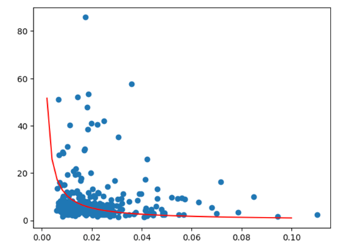
Figure 1: The scatter plot of degree of freedom (y-axis) and standard deviation (x-axis)

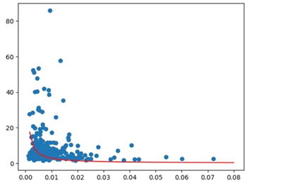
Figure 2: the scatter plot of degree of freedom (y-axis) and \( \frac{interquatile range}{mean} \) (x-axis)

All these graphs’ x axis is degree of freedom and y axis is the fluctuation of stock returns. We can see that these two variables have inverse relationship which prove our ideas.

8. Conclusion

The essay shows that the degree of freedom has a inverse relationship with the fluctuation of the stock. In summary, this academic essay provides empirical evidence supporting the assertion that the student’s t-distribution offers a superior fit when compared to the normal distribution for modeling stock returns. Additionally, the essay underscores the efficiency of employing Maximum Likelihood Estimation (MLE) as a suitable method for estimating the parameters of both the student’s t-distribution and the normal distribution in this context. Lastly, the study illuminates a noteworthy finding, indicating an inverse relationship between the degree of freedom and the volatility of stock returns.

References

[1]. Hayes, A. (n.d.). What is T-distribution in probability? how do you use it?. Investopedia. https://www.investopedia.com/terms/t/tdistribution.asp#:~:text=The%20Bottom%20Line-,The%20t%2Ddistribution%20is%20used%20in%20statistics%20to%20estimate%20the,greater%20chance%20for%20extreme%20values.
[2]. Rossi, Richard J. (2018). Mathematical Statistics: An Introduction to Likelihood Based Inference. New York: John Wiley & Sons. p. 227. ISBN 978-1-118-77104-4.
[3]. What are logarithmic returns and how to calculate them in pandas dataframe. Saturn Cloud Blog. (2023, September 8). https://saturncloud.io/blog/what-are-logarithmic-returns-and-how-to-calculate-them-in-pandas-dataframe/#:~:text=Logarithmic%20returns%2C%20also%20known%20as,the%20value%20of%20an%20asset.
[4]. Clauset, A., Shalizi, C. R., & J., N. M. E. (2009). 3.3. In Power-law distributions in empirical data. essay, Arxiv.
[5]. Huelsenbeck, J. P., Hillis, D. M., & Nielsen, R. (1996). A likelihood-ratio test of monophyly. Systematic Biology, 45(4), 546–558. https://doi.org/10.1093/sysbio/45.4.546
Cite this article
Xiao,N.;Shi,W. (2024). Do Stock Returns Adhere to the Distribution Stipulated by the Student’s T-distribution?. Advances in Economics, Management and Political Sciences,92,233-239.
Data availability
The datasets used and/or analyzed during the current study will be available from the authors upon reasonable request.
Disclaimer/Publisher's Note
The statements, opinions and data contained in all publications are solely those of the individual author(s) and contributor(s) and not of EWA Publishing and/or the editor(s). EWA Publishing and/or the editor(s) disclaim responsibility for any injury to people or property resulting from any ideas, methods, instructions or products referred to in the content.
About volume
Volume title: Proceedings of the 2nd International Conference on Financial Technology and Business Analysis
© 2024 by the author(s). Licensee EWA Publishing, Oxford, UK. This article is an open access article distributed under the terms and
conditions of the Creative Commons Attribution (CC BY) license. Authors who
publish this series agree to the following terms:
1. Authors retain copyright and grant the series right of first publication with the work simultaneously licensed under a Creative Commons
Attribution License that allows others to share the work with an acknowledgment of the work's authorship and initial publication in this
series.
2. Authors are able to enter into separate, additional contractual arrangements for the non-exclusive distribution of the series's published
version of the work (e.g., post it to an institutional repository or publish it in a book), with an acknowledgment of its initial
publication in this series.
3. Authors are permitted and encouraged to post their work online (e.g., in institutional repositories or on their website) prior to and
during the submission process, as it can lead to productive exchanges, as well as earlier and greater citation of published work (See
Open access policy for details).