1. Introduction

Recent advancements in portfolio management emphasize the necessity of dynamic and robust optimization techniques, especially in response to the increasing volatility observed in global markets. Traditional models, such as those incorporating the Upper Confidence Bound (UCB) and Kullback-Leibler Upper Confidence Bound (KL-UCB) algorithms [1], have predominantly focused on static settings without sufficient mechanisms for adjustment under market stress. These approaches often overlook the complex interdependencies of modern financial markets and fail to incorporate advanced computational methods that can enhance predictive accuracy and risk management [2].

This paper aims to bridge these gaps by introducing sophisticated methods for portfolio construction and analysis [3]. By integrating convex optimization and Monte Carlo simulation, it offers a nuanced approach that allows for detailed assessments of risk and return, aligning with the complexities of contemporary investment strategies [4]. Specifically, the work extends the functionality of the KL-UCB algorithm to accommodate dynamic weight adjustments, providing a significant improvement in handling periods of high market volatility [5]. Moreover, the research advances the discourse on risk and leverage management by incorporating these elements into a cohesive strategy tailored to diverse investor profiles [6-7]. The empirical analysis and backtesting presented herein not only underscore the practical application of our methods but also demonstrate their superiority in real-market scenarios compared to more conventional models [8-10].

This introduction adheres to the guidelines set forth by the journal, ensuring that the manuscript is prepared for submission without the need for re-typing. The subsequent sections will delve into the model formulation, and detailed application processes, and discuss the theoretical and practical implications of the findings.

2. Model Formulation

2.1. The basic fundamental of MAB and KL-UCB Algorithm

The Multi-Armed Bandit (MAB) algorithm is a decision-making algorithm used to make a series of choices in an uncertain environment to maximize total rewards. It originates from the problem of playing slot machines, where one machine may have multiple levers (arms), each with a different unknown probability distribution of rewards. Pulling an arm constitutes a trial, and the objective is to obtain as many rewards as possible within a finite number of trials.

The core challenge of the Multi-Armed Bandit (MAB) algorithm revolves around the strategic balance between exploration and exploitation. Exploration involves testing different arms to accumulate data about their reward probabilities, which is essential for uncovering potentially higher-yielding options. Conversely, exploitation capitalizes on this gathered information by selecting the arm that has historically provided the best returns, thereby maximizing rewards. This dynamic interplay aims to optimize decision-making processes by carefully weighing the potential benefits of discovering new opportunities against the advantages of leveraging known outcomes. No fixed formula describes all MAB algorithms since there are multiple strategies. However, the common objective of all strategies is to maximize the total rewards, typically represented as:

(1)

where:

is the total reward and

is the total number of periods.

is the reward obtained by pulling the arm

at a time

.

The KL-UCB algorithm offers a refined strategy for the multi-armed bandit (MAB) problem, aiming to maintain a balance between exploration and exploitation. This approach involves determining a confidence upper bound for each option, or "arm," at every decision point. The algorithm then proceeds to select the arm with the highest upper bound, reflecting the most promising potential reward given past performances and uncertainties. The critical aspect of KL-UCB is the computation of these bounds, which are derived through an optimization process. Specifically, the upper bound for each arm is calculated by solving an optimization problem that estimates the most optimistic potential outcome for that arm, based on the data accumulated up to that time. This calculates upper bound guides the selection process, steering decisions towards either exploiting a well-performing arm or exploring less tried arms that might offer greater rewards.

(2)

where:

is the confidence upper bound a time

.

is the number of times an arm

has been selected up to time

.

is the empirical success probability of arm

up to time

. KL(p, q) is the Kullback-Leibler divergence between two probabilities

, and

. c is a positive parameter that adjusts the level of exploration.

Kullback-Leibler divergence is an asymmetric measure of the difference between two probability distributions, defined as:

(3)

In this context,

is typically the actual success probability of

the arm, while

is the value we are seeking, representing an upper bound on the estimated success probability at time

.

2.2. The establishment of the Fama-French Three-Factor Model

The Fama-French Three-Factor Model analysis conducted in this report is rooted in the understanding that the returns of a portfolio are influenced by various systematic risk factors. These factors are believed to capture the majority of the diversifiable risk of a portfolio and are used to explain the returns above and beyond what can be explained by the market risk alone. The model postulates that the expected return of a portfolio over the risk-free rate (excess return) can be explained by its sensitivity to three factors: Market Risk Premium (Mkt-RF) represents the additional return investors require for investing in stocks compared to risk-free securities. Size Premium (SMB) captures the excess return of small-cap stocks over large-cap stocks, while Value Premium (HML) represents the excess return of value stocks over growth stocks.

The linear regression model to estimate the coefficients that describe the relationship between these factors and the portfolio returns is represented as follows:

(4)

Where:

is the return of the portfolio at time

,

is the risk-free rate at time

,

is the return of the market portfolio at time

.

is the intercept, representing the portfolio's excess return that is not explained by the model.

These are the sensitivities of the portfolio to the market excess return, size premium, and value premium, respectively.

is the error term of the regression at time

.

2.3. Portfolio Construction and Efficient Frontier Analysis

2.3.1. Application of Monte Carlo Simulation in Portfolio Analysis

Monte Carlo simulation is a statistical simulation technique used to estimate the probability distribution characteristics of complex systems. In portfolio management, it is used to generate potential asset allocations and calculate the expected returns, volatility (standard deviation), and Sharpe ratio of these allocations.

Construction process:

Firstly, prepare the data by gathering historical return data for the assets you want to analyze, as this is crucial for estimating the expected returns and volatility of each asset.

Simulating asset weights:

(5)

Where

is a random number for the

asset.

Then, simulate various asset weights by generating random numbers for each asset, ensuring that the sum of all weights equals one. In the second step, calculate the expected portfolio return using the formula.

Expected portfolio return

:

(6)

Portfolio volatility

:

(7)

where

is the vector of asset returns,

is the covariance matrix, and

is the weight vector.

Finally, repeat this simulation multiple times—commonly 100,000 iterations—to generate a broad range of potential portfolios. This extensive simulation helps in plotting the efficient frontier, which visually depicts the trade-off between portfolio risk and return, allowing investors to choose portfolios that align with their risk tolerance and return objectives.

2.3.2. Building the Efficient Frontier Using SciPy for Portfolio Optimization

SciPy can solve optimization problems to find asset allocations that provide maximum expected returns at different levels of risk or minimize volatility.The process for constructing an optimized investment portfolio involves several key steps, aimed at either minimizing volatility or maximizing the Sharpe ratio under given constraints.

Firstly, the objective is set to minimize portfolio volatility, subject to constraints such as achieving a specific target return and ensuring the sum of asset weights equals one.

Minimize volatility:

(8)

Constraints:

(target return),

(sum of weights equals one).

Secondly, the objective shifts to maximizing the Sharpe ratio, again subject to appropriate constraints.

Maximize Sharpe ratio:

(9)

Constraint:

The third step involves solving the optimization problem, Finally, the results of this optimization are analyzed to determine the optimal asset allocations that meet different target returns or desired risk levels, thereby guiding investment decisions.

2.3.3. Constructing Efficient Frontier through Convex Optimization Techniques

Convex optimization is a special mathematical optimization method used to handle optimization problems with convex functions or convex constraints. In portfolio theory, convex optimization is used to find the optimal trade-off between risk and return.

To construct an optimized investment portfolio, it begins by formulating an optimization problem.

The objective function aims to maximize the expected return of the portfolio adjusted by a risk aversion coefficient, while minimizing the portfolio's risk. This balancing act of risk and return forms the crux of the optimization. It imposes necessary constraints to ensure the solution is practical, such as those on the sum of asset weights.

Objective function:

(10)

where

are the risk aversion coefficient,

the expected return of the portfolio, and

the risk of the portfolio.

Constraint:

Next, it employs convex optimization techniques using libraries like cvxpy to solve this problem, allowing us to determine the optimal asset allocations that balance risk and return efficiently. Finally, it explores the role of leverage in portfolio optimization. By varying leverage levels, it analyzes how they expand the range of achievable risk and return profiles on the efficient frontier, potentially enhancing the portfolio's performance under different market conditions.

3. Results

3.1. Analysis of MAB and KL-UCB Algorithm

The study examined how dynamic weight adjustments using the KL-UCB algorithm can optimize asset management. This part of the analysis focused on observing asset weight changes over time within an investment portfolio.

Through using the model, it can get the following results:

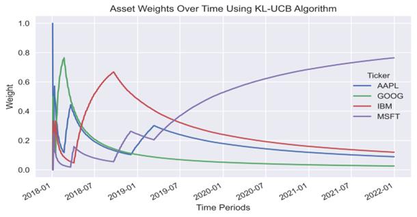
Figure 1: Asset Weights over time

The Figure 1 shows distinctive trends. AAPL initially holds a dominant weight, which decreases sharply, suggesting an initial overestimation of its returns, but it later begins to rise again. GOOG (Alphabet Inc. - Google) consistently increases in weight, eventually becoming the most heavily weighted asset. IBM's weight quickly declines to near zero, indicating its poor performance relative to other assets. MSFT (Microsoft Corporation) experienced a significant mid-term increase in 2020 due to strong market performance but later decreased as the weight shifted towards GOOG, reflecting the algorithm's adaptation to market changes.

It aims to analyze and compare the performance of two different investment portfolio strategies: one based on a reference portfolio with balanced asset allocation (referred to as the "Reference Portfolio"), and the other utilizing a dynamic weight adjustment strategy (referred to as the "Strategy Portfolio"). The weight adjustment in the Strategy Portfolio is based on the KL-UCB algorithm, which dynamically adjusts the weights of assets in the portfolio based on their historical performance. For comparison purposes, we calculate the cumulative returns of both portfolios and present them on the same chart.

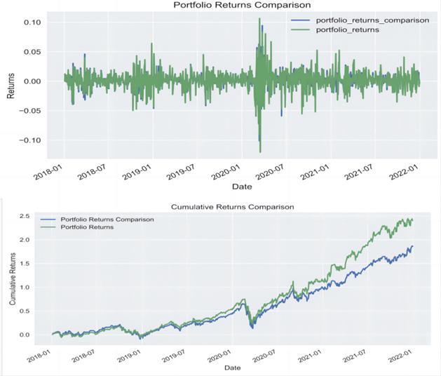
Figure 2: Portfolio and Cumulative returns

By observing Figure 2, it can be observed that especially during the market volatility in early 2020, the Strategy Portfolio exhibits better resilience compared to the Reference Portfolio. This may be attributed to the KL-UCB algorithm continuously adjusting the weights and effectively capturing the market rebound, leading to the allocation of funds accordingly.

KL-UCB algorithm demonstrates an advantage over the Reference Portfolio in terms of overall returns, particularly during periods of significant market fluctuations. This finding highlights the potential value of utilizing dynamic weight adjustment strategies in asset management. The data and analysis results presented in this report provide investors with valuable insights, indicating that by leveraging advanced algorithms such as KL-UCB, portfolio performance can be optimized effectively in complex market environments.

3.2. Analysis of the Fama-French Three-Factor Model:

This section evaluated how well the Fama-French three-factor model explains the returns of the portfolio, focusing on the impact of market risk premium, size premium, and value premium.

Regression Statistics:

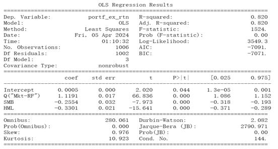
Figure 3: OLS Regression Results

The Figure 3 effectively captures the dynamics of the portfolio's returns, as indicated by the high R-squared value of 0.82, which shows that the model accounts for a significant portion of the variation in the portfolio's excess returns. The statistical robustness of the model is further underscored by a high F-statistic of 1524 and a near-zero p-value, highlighting its significance. The analysis of regression coefficients reveals that the portfolio has a strong positive relationship with market movements, as evidenced by the Market Risk Premium coefficient of 1.1191. This suggests that a 1% increase in the market yields approximately a 1.1191% increase in the portfolio's performance, reflecting high market sensitivity. In contrast, the coefficients for Size Premium and Value Premium, at -0.2554 and -0.3301 respectively, show that small-cap and value stocks negatively impact the portfolio's excess returns, with value stocks having a more substantial detrimental effect. This rolling regression analysis provides crucial insights into how different market factors influence the portfolio over time, shedding light on its performance characteristics.

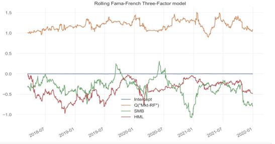
Figure 4: Rolling Fama-French Three-Factor model

The Figure 4 provides insightful trends in the coefficients over time. The intercept, though volatile, stays close to zero across different periods, suggesting minimal unexplained variance in the model. The market risk premium (Mkt-RF) coefficient shows strong positive fluctuations, underscoring its significant influence on the portfolio's performance across various market conditions. Conversely, the coefficients for SMB (size premium) and HML (value premium) generally exhibit a negative correlation, highlighting a strategic preference for large-cap growth stocks within the investment portfolio. This analysis illustrates how different market factors dynamically affect the investment strategy's returns.

The regression analysis showed a high R-squared value of 0.82, indicating that the model effectively captures the variations in the portfolio's excess returns. The market risk premium was identified as a significant positive influencer, while size and value premiums negatively affected the portfolio, suggesting a bias towards large-cap growth stocks. The rolling regression analysis highlighted how these factor sensitivities varied over time.

3.3. Analysis of Convex Optimization Techniques:

This section investigated the use of convex optimization techniques and Monte Carlo simulations to determine the optimal asset allocation for maximizing returns and minimizing volatility.

3.3.1. Monte Carlo simulation

Monte Carlo simulation is a statistical simulation technique used to estimate the probability distribution characteristics of complex systems. In portfolio management, it is used to generate potential asset allocations and calculate the expected returns, volatility (standard deviation), and Sharpe ratio of these allocations.

To use Monte Carlo simulation to find the efficient frontier, it first calculates the stock prices of the considered assets and daily returns of the considered assets.

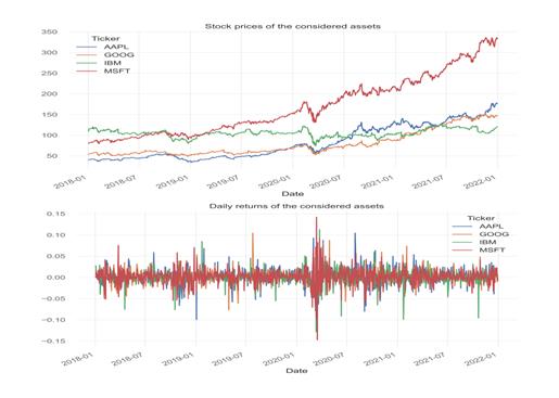
Figure 5: Stock prices and Daily returns

The figure 5 illustrates the price trends and daily return distribution of four stocks. And then it shows the frontier:

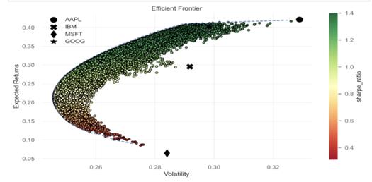
Figure 6: Efficient Frontier

The Figure 6 displays a scatter plot of a Monte Carlo simulation, showcasing the expected returns (Y-axis) and volatility (X-axis) of various investment portfolios. The color of the dots represents the Sharpe ratio. The curve in the scatter plot represents the efficient frontier, which is the set of investment portfolios that offer the maximum expected returns for a given level of risk. Dots above the efficient frontier represent portfolios with higher risk but higher expected returns.

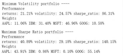
Figure 7: Min and Max Sharpe Ratio portfolio

The Figure 7 present the performance and weight allocation of two specific investment portfolios. One is the portfolio with the maximum Sharpe ratio, and the other is the portfolio with the minimum volatility. The portfolio with the maximum Sharpe ratio has an expected return of 40.89%, volatility of 29.18%, and a Sharpe ratio of 1.40 (or 140.15%), indicating higher expected excess returns for each unit of total risk undertaken. The weight allocation shows that this portfolio is primarily invested in AAPL and GOOG, accounting for over 98% of the total investment. The portfolio with the minimum volatility has an expected return of 21.21%, volatility of 24.57%, and a Sharpe ratio of 0.86 (or 86.31%), indicating a relatively conservative portfolio primarily invested in MSFT and IBM.

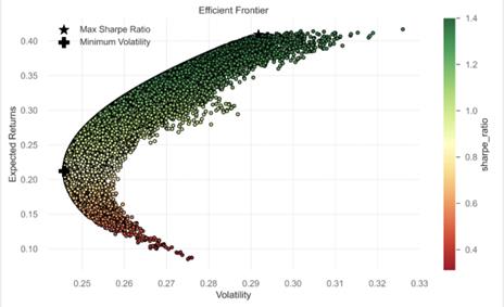
Figure 8: Efficient Frontier

The Figure 8 highlights the positioning of these two specific investment portfolios on the scatter plot, showcasing how they perform about other potential portfolio allocations.

The simulation helped plot an efficient frontier, showing various potential investment portfolios' expected returns against their volatility. The analysis highlights portfolios that optimize the risk-return trade-off.

3.3.2. SciPy for Portfolio Optimization

Using the optimization function "minimize" from SciPy, a series of investment portfolios is generated to construct the efficient frontier by finding the weights of each asset that minimize volatility for a given range of target returns. These portfolios have the lowest possible risk at the specified expected return levels. They are ideal choices for investors aiming to optimize investment returns at specific risk levels. The results are as follows:

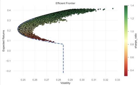
Figure 9: Efficient Frontier

According to the Figure 9, it can be concluded that:

The minimum volatility portfolio aims to minimize the investment's fluctuations while still offering a reasonable return. It achieves a return of 21.42% with a volatility of 24.57% and a Sharpe ratio of 87.15%. The portfolio's stock weight allocation is as follows: AAPL accounts for 11.10%, IBM for 30.47%, MSFT for 46.63%, and GOOG for 11.79%. This allocation strategy ensures that MSFT has the highest weighting in the portfolio, while GOOG and AAPL have smaller proportions, and IBM holds the second-largest allocation.

The Maximum Sharpe Ratio portfolio is designed to maximize excess returns relative to volatility (measured by the Sharpe ratio) after adjusting for the risk-free rate. With a return of 40.92% and a volatility of 29.14%, it achieves an impressive Sharpe ratio of 140.40%. The stock weight allocation for this portfolio is as follows: AAPL accounts for 38.71%, IBM 0.00%, MSFT 0.00%, and GOOG 61.29%. Notably, the majority of the portfolio's weight is allocated to GOOG and AAPL, totaling almost 100%. This indicates that the strategy of the Maximum Sharpe Ratio portfolio is to concentrate investments in assets expected to deliver optimal performance.

3.3.3. Convex Optimization Techniques

This model maximizes the investment portfolio's return based on the average return and covariance matrix while subtracting a term associated with risk (regulated by γ). The optimization problem is solved using covariance programming (using the copy library), iterating through different γ values to obtain optimal investment portfolio weights at different risk aversion levels.

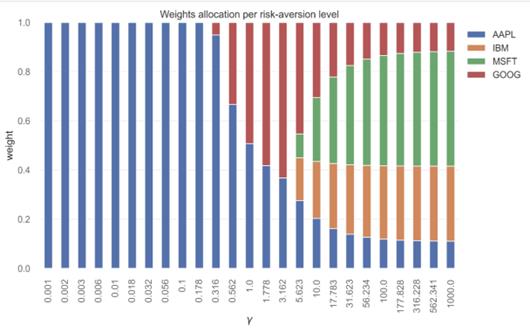
Figure 10: Weights allocation per risk-aversion level

The model considers different levels of risk aversion. In the Figure 10, the x-axis represents the risk aversion coefficient (denoted as γ), which is on a logarithmic scale ranging from very low (almost no risk aversion, more inclined towards pursuing high returns) to very high (extreme risk aversion, more inclined towards safe investments). The y-axis represents the weights allocated to each asset, with a total sum of 1. As the risk aversion coefficient increases, It can observe how the weights of different assets in the investment portfolio change. When the risk aversion coefficient is very low, the model tends to allocate the investment solely to one asset (in this case, AAPL). However, as the risk aversion coefficient increases, the investment gets diversified into other assets, which is often considered a more conservative investment strategy with greater risk diversification.

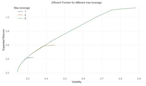
Figure 11: Efficient Frontier for different max leverage

The Figure 11 depicting the efficient frontier demonstrates how investment portfolios perform under varying levels of maximum leverage, illustrating the trade-offs between risk and return. With a leverage of 1, the frontier shows portfolios that balance lower risk and return. As leverage increases to 2, the frontier shifts upward and to the right, suggesting that portfolios can secure higher returns at the cost of taking on more risk. The trend intensifies with a maximum leverage of 5, where the frontier moves even further right, indicating the potential for even higher returns, albeit paired with significantly increased risk. This progression highlights the direct correlation between leverage levels and both potential returns and associated risks in portfolio management.

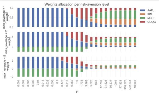
Figure 12: Weights allocation per risk-aversion level

The Figure 12 showcasing asset weight allocation under different levels of maximum leverage and varying degrees of risk aversion, represented by the coefficient γ, reveals how investment strategies adjust based on risk preferences. At a leverage of 1, with low γ indicating minimal risk aversion, portfolios are highly concentrated in specific assets like AAPL. However, as γ increases, indicating heightened risk aversion, asset allocation becomes more diversified to mitigate risk. When leverage rises to 2 and then to 5, asset weight shifts become more pronounced, with even negative weights emerging at the highest leverage, suggesting the use of short positions to hedge or leverage risks associated with other investments. This dynamic illustrates how portfolios adapt to balance return objectives against risk tolerance, particularly as leverage and risk aversion levels change.

The application of the copy library helped in optimizing the portfolio by varying levels of risk aversion, showing how asset weights adjusted according to different risk preferences, and further expanded on this by adjusting levels of leverage to explore wider ranges of risk-return combinations.

4. Conclusions

The Strategy Portfolio utilizing the KL-UCB algorithm showcases superior overall returns compared to the Reference Portfolio, especially during significant market fluctuations, underscoring the effectiveness of dynamic weight adjustment strategies in asset management. Analysis with the Fama-French three-factor model reveals the market risk premium as the main driver of the portfolio's excess returns, with negative impacts from size and value premiums suggesting a preference for large-cap growth stocks. These insights advocate for ongoing risk monitoring and strategic adjustments, particularly against SMB and HML factors. Additionally, portfolios with different Sharpe ratios highlight the trade-offs between expected returns and volatility, affecting investor choices based on risk appetite. The use of leverage, as demonstrated, increases both potential returns and associated risks, indicating that while higher leverage can enhance returns, it also requires careful risk management. Moderate leverage levels, such as a maximum of 2, offer a balanced approach between risk and return, emphasizing the need for tailored investment strategies that align with individual risk preferences and market conditions.

References

[1]. Sun, Y. Portfolio Strategy Based on Multifactor Models and Multi-Armed Bandit Algorithm(in Chinese) [D]. Shandong University, 2022. DOI: 10.27272/d.cnki.gshdu.2022.006035.
[2]. Yuan, S. Research and Implementation of Portfolio Analysis System Based on Deep Reinforcement Learning (in Chinese) [D]. Ningxia University, 2020. DOI: 10.27257/d.cnki.gnxhc.2020.000716.
[3]. Miao, M. Application Research of Multifactor Stock Selection Model in Portfolio Management (in Chinese) [D]. Nanjing Audit University, 2018.
[4]. Xie, H., Hu, D. Application of Multifactor Quantitative Model in Portfolio: A Comparative Study Based on LASSO and Elastic Net (in Chinese). Statistics and Information Forum, 2017, 32(10): 36-42.
[5]. Qin X, Shi P, Ye Z. Research On Portfolio Construction for Information Technology and Communication Service Industries Based on The Monte Carlo Simulation[A]. Wuhan Zhicheng Times Cultural Development Co., Ltd..Proceedings of 2022 International Conference on Financial Technology and Market Management (FTMM 2022)[C].Wuhan Zhicheng Times Cultural Development Co., 2022:9.DOI:10.26914/c.cnkihy.2022.085188.
[6]. Li, S. Implementation of Financial Applications Based on Python Scientific Computing Packages (in Chinese) [D]. Jiangxi University of Finance and Economics, 2017.
[7]. Hou, L. Several Algorithms for Nonsmooth Convex Optimization (in Chinese) [D]. Nanjing Normal University, 2007.
[8]. Cai, X. Research on Some Splitting Algorithms for Convex Optimization and Monotone Variational Inequalities and Their Computational Complexity (in Chinese) [D]. Nanjing University, 2013.
[9]. Yan Z, Jiyuan T, Zhixiang Y, et al. Improved Large Covariance Matrix Estimation Based on Efficient Convex Combination and Its Application in Portfolio Optimization[J]. Mathematics,2022,10(22).
[10]. Davi V M, Álvaro V, Alexandre S. A Linear Stochastic Programming Model for Optimal Leveraged Portfolio Selection[J]. Computational Economics,2018,51(4).
Cite this article
Qiu,H. (2024). Investment Portfolio with Convex Optimization and Risk Adjustment Using Multi-Factor Model and Multi-Armed Bandit Algorithm. Advances in Economics, Management and Political Sciences,104,55-68.
Data availability
The datasets used and/or analyzed during the current study will be available from the authors upon reasonable request.
Disclaimer/Publisher's Note
The statements, opinions and data contained in all publications are solely those of the individual author(s) and contributor(s) and not of EWA Publishing and/or the editor(s). EWA Publishing and/or the editor(s) disclaim responsibility for any injury to people or property resulting from any ideas, methods, instructions or products referred to in the content.
About volume
Volume title: Proceedings of the 8th International Conference on Economic Management and Green Development
© 2024 by the author(s). Licensee EWA Publishing, Oxford, UK. This article is an open access article distributed under the terms and
conditions of the Creative Commons Attribution (CC BY) license. Authors who
publish this series agree to the following terms:
1. Authors retain copyright and grant the series right of first publication with the work simultaneously licensed under a Creative Commons
Attribution License that allows others to share the work with an acknowledgment of the work's authorship and initial publication in this
series.
2. Authors are able to enter into separate, additional contractual arrangements for the non-exclusive distribution of the series's published
version of the work (e.g., post it to an institutional repository or publish it in a book), with an acknowledgment of its initial
publication in this series.
3. Authors are permitted and encouraged to post their work online (e.g., in institutional repositories or on their website) prior to and
during the submission process, as it can lead to productive exchanges, as well as earlier and greater citation of published work (See
Open access policy for details).