1. Introduction

In the inherently uncertain environment of financial markets, characterized by drastic fluctuations in the prices of stocks, bonds, commodities, and other assets, portfolio management serves as a crucial mechanism for investors to oversee their assets actively. Performing a comprehensive return and risk analysis is indispensable to navigate through volatility [1]. By judiciously allocating assets in a portfolio, investors strategically optimize their investments by maximizing returns following their risk tolerances. Thus, portfolio optimization is an essential component of financial management. Constructing a successful portfolio is important not only in improving investment outcomes but also in mitigating investment risks [2]. Therefore, the pursuit of optimal portfolio strategies is pivotal in both academic research and practical financial applications.

Harry Markowitz developed Modern Portfolio Theory, which forms the foundation of contemporary portfolio management. He introduced the revolutionary concept of efficient frontier, a curve representing portfolios delivering the highest potential returns for specific risk amounts and the lowest risk for a designated return expectation. This mean-variance optimization framework shifted the focus from individual asset selection to the holistic composition of portfolios. Markowitz articulated that an effective portfolio is not merely a collection of good assets but a balanced whole that renders investors protection and opportunities across various circumstances [3].

Extensive research has been made in the area of portfolio optimization, to address the limitations of the traditional Mean-Variance (MV) model introduced by Markowitz. Kalayci and Ertenlice extensively reviewed 175 papers, highlighting efforts to refine the MV model by incorporating real-time conditions and developing various model variants [4]. Chen et al. utilized swarm intelligence algorithms to address complex challenges in portfolio optimization [1]. To address the estimation issue when applying portfolio optimization models to real data, Ban et al. put forward a performance-based regularization (PBR) function that helps reduce estimation error [5]. Lee and Kim introduced two innovative sparse and robust portfolio selection models. Their approach involves an initial semi-definite relaxation followed by an extension using L2 norm regularization [6]. Zhang, Li, and Guo critically examined the variations of the mean-variance portfolio model, particularly addressing the limitation to adapt to the constantly dynamic financial market and operational challenges in practice. The robust portfolio optimization, fuzzy portfolio optimization, and dynamic portfolio optimization are developed to offset the limitations. They also suggested that combining predictive models with portfolio optimization presents a promising approach for future research to mitigate risk and manage uncertainty [7].

Indeed, many studies in recent years demonstrated that machine learning models are feasible tools to forecast dynamic movement in the financial market. It excels in capturing non-linear patterns with ensemble learning [8]. Algorithms including the Random Forest Model and Deep Neural Networks are utilized to predict stock prices and integrated to implement stock selection [9]. Nevertheless, while the integration of machine learning models into portfolio optimization shows promise, it is still insufficiently explored, highlighting significant potential for further research. Following Zhang’s research, this study aims to integrate forecasts with portfolio optimization techniques to formulate effective asset allocation strategies.

To achieve this objective, the study begins by selecting nine assets from diverse sectors, thereby constructing a diversified investment portfolio. It utilizes historical data spanning three quarters as a training set in forecast models, employing a rolling window approach to predict the returns of individual assets for the subsequent quarter. According to the Mean-Variance Portfolio theory, the study subsequently leverages Monte Carlo simulations to identify and visualize the Efficient Frontier, in order to determine the asset allocation strategy in optimal portfolios that deliver the maximum Sharpe Ratio or minimized volatility. For model validation, the optimal weights are applied to the historical returns of the individual assets in the next quarter. The performance metrics of these portfolios are then computed and compared with each other and against S&P 500 index’s performance. This validation through backtesting with actual market data enhances the credibility of the forecasting and optimization techniques used, demonstrating their practical applicability and robustness in a real investment context.

2. Methodology

2.1. Data Collection

Following the principle of diversification, this paper selects eight assets from different sectors (See Table 1).

Table 1: Selected stocks

The dataset consists of historical price data for eight selected assets and the S&P 500, which serves as a representative indicator of the market for the later comparative performance evaluation. The data originate from Yahoo Finance (https://finance.yahoo.com/) and span from June 1, 2023, to June 1, 2024. Instead of the standard closing price, the analysis is based on the adjusted close price as it accounts for corporate decisions like stock splits and dividends. Using the adjusted close prices ensures that the returns calculated are true reflections of investors’ profits. Compounded returns(log-return) for each asset are computed, according to the following formula.

\( \text{C}_{\text{t}}\text{ =ln (}\frac{\text{V}_{\text{t}}\text{ }}{\text{V}_{\text{t-1}}}\text{)} \) (1)

Table 2 illustrates the descriptive data of compounded return of considered assets.

Table 2: Descriptive data of compounded return of considered assets

Notably, PGR (0.0020) and COST (0.0019) have the highest mean compounded returns among the considered assets, suggesting relatively better average performance. FSLR (0.0293) and NFLX (0.0218) have the highest standard deviations, indicating higher risk associated with these assets. In contrast, GOOGL (0.0018) has the lowest standard deviation, suggesting it is the least volatile asset. Skewness provides insights into the asymmetry of return distributions. PGR (-1.605) has a significantly negative skewness, indicating a tendency for extreme negative returns. Conversely, FSLR (1.226) and GE (1.104) exhibit positive skewness, suggesting a propensity for extreme positive returns. ​​ Kurtosis measures the “tailedness” of the return distribution. PGR (24.831) and NFLX (11.082) have extremely high kurtosis values, implying the presence of extreme outliers. This indicates a higher likelihood of experiencing extreme returns, both positive and negative.

2.2. Forecast: Rolling Window Approach

The rolling window approach is a robust method employed for forecasting stock returns, particularly effective for time series analysis in dynamic environments such as financial markets. This method utilizes a fixed-size segment of historical data, termed a “window,” to continuously train and update forecasting models. Specifically, the dataset, consisting of historical returns from 252 trading days, is separated into a training set (189 trading days) and a validation set (63 days).

The process updates training set daily. After predicting the next day’s return, the model integrates this newly estimated data point and discards the oldest data. The window slides forward incrementally by one day at a time, with the model being re-trained with each shift. The process continues until the window reaches the end of the forecast horizon. It enables the model to generate accurate predictions based on its previous forecasts [10].

The purpose of including estimated return rather than actual return in the training process is to maintain an unbiased evaluation of the model. Beyond mere backtesting, the primary aim is not to perfect daily predictions—which is impractical for daily portfolio adjustments—but rather to determine optimal portfolio weights based on estimated returns. This approach aligns with the practical demands of portfolio management, emphasizing long-term performance and risk mitigation over short-term market fluctuations.

2.3. Light Gradient Boosting Machine

Researchers have validated the effectiveness of LightGBM in predicting short-term stock volatility [11]. A comparative study by Hartanto et al. illustrates that LightGBM outperforms other boosting-based forecasting models such as XGBoost and CatBoost in projecting stock prices [12]. Motivated by these findings, this study employs the LightGBM model optimized by Optuna. It dynamically inputs values for various hyperparameters within specified ranges, trains the model and iteratively adjusts the parameters based on lower root mean squared error (RMSE). This optimization process aims to refine the model parameters to minimize the RMSE of predictions.

Given that gradient boosting utilizes tree-based learning algorithms, LightGBM is recognized for its faster training speed and higher accuracy. It addresses the limitation of traditional gradient-boosting decision trees by incorporating a gradient-based one-sided sampling method to split trees. This technique not only reduces memory usage but also enhances efficiency and accuracy, particularly in scenarios with large and imbalanced datasets (See Figure 1).

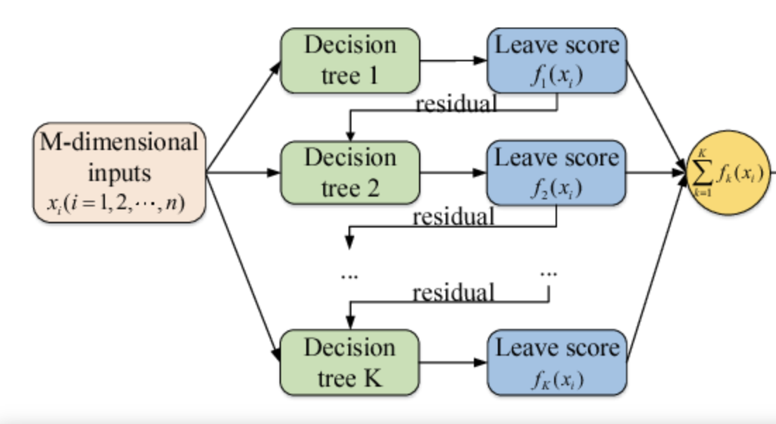
Figure 1: Flowchart of Light Gradient Boosting Machine model [13]

The diagram shows how each decision tree (Tree 1, Tree 2, …, Tree K) is built sequentially, with each tree learning from the residuals of the previous tree. Each tree produces a leaf score based on the inputs. The summing of leaf scores across all trees to produce a final predicted value. Such aggregation combines the incremental improvement from all the trees. The flow from multidimensional inputs through trees to a cumulative output illustrates how LightGBM keeps improving prediction from iterations.

2.4. Random Forest

This study utilizes the Random Forest model to project the compounded returns of individual stocks. The model is fine-tuned using GridSearchCV to identify optimal parameters, which are then used to evaluate the model’s performance via RMSE on a test set. Subsequently, the model is employed in a rolling prediction approach, where it iteratively forecasts future returns by including the newly estimated data points and removing the most outdated entry. The Random Forest model is considered as a robust machine learning technique that employs a collection of multiple decision trees to carry out tasks such as classification and regression (See Figure 2).

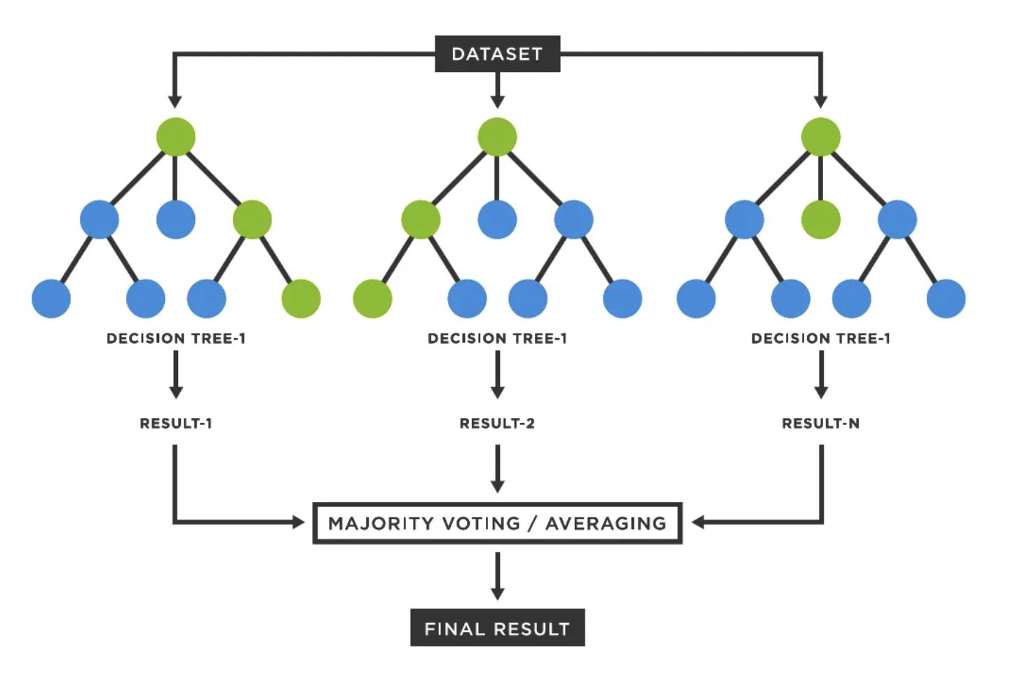
Figure 2: Illustration of Random Forest Model

As Figure 2 shows, the Random Forest (RF) model is an ensemble method comprising numerous trees whose collective decisions determine the outcome. Decisions are aggregated through either majority voting or averaging, to improve performance and avoid overfitting, which are the major advantages of the Random Forest approach. The empirical research by Basak et al. establishes a model that leverages random forest and gradient-boosted decision trees to forecast stock price movements. It concludes that random forest is preferred because it employs a substantial number of independent decision trees and aggregates predicting through a voting mechanism, making it particularly effective in the stock market context [14].

2.5. Mean-Variance Portfolio

In Mean-Variance Portfolio theory, portfolios are evaluated on two dimensions: the expected return and risk, or the variance of return. The Efficient Frontier visually delineates the collection of portfolios that optimally balance the tradeoff between risk and return. Markowitz presents the Monte Carlo simulation as a powerful tool in portfolio optimization. By simulating numerous random portfolios with distinct weight allocations, investors can estimate the distribution of returns and risks, thereby allowing them to identify the portfolios lying on the Efficient Frontier. It is visualized as an upward-sloping curve, indicating the positive correlation between risk and return. Inside the Markowitz model, three indicators are crucial for the optimization: expected return, volatility, and Sharpe Ratio. These indicators are formulated below.

This metric is computed by aggregating the expected returns of each constituent asset in the portfolio, weighted according to their allocation proportions. Mathematically, it is represented as:

\( \text{E(}\text{R}_{\text{p}}\text{) =}\sum _{\text{i=1}}^{\text{n}} \text{w}_{\text{i}}\text{ E(}\text{R}_{\text{i}}\text{)}\text{ = }\sum _{\text{i=1}}^{\text{n}} \text{w}_{\text{i }}\text{μ}_{\text{i }} \) (2) \( \text{E(}\text{R}_{\text{p}}\text{) =}\sum _{\text{i=1}}^{\text{n}} \text{w}_{\text{i}}\text{ E(}\text{R}_{\text{i}}\text{)}\text{ = }\sum _{\text{i=1}}^{\text{n}} \text{w}_{\text{i }}\text{μ}_{\text{i }} \)

The portfolio’s risk is measured by volatility, or the variance of the portfolio’s expected return. It is calculated by summing the products of the weights and covariances of all pairs of assets, as the following shows:

\( \text{σ}_{\text{p}}^{\text{2}}\text{ =var (}\sum _{\text{i=1}}^{\text{n}} \text{w}_{\text{i}}\text{ E(}\text{R}_{\text{i}}\text{)}\text{) =}\sum _{\text{i=1}}^{\text{n}} \sum _{\text{j=1}}^{\text{n}} \text{w}_{\text{i}}\text{w}_{\text{j}}\text{ cov(}\text{r}_{\text{i}}\text{r}_{\text{j}}\text{)} \) (3)

The Sharpe Ratio helps in understanding how much additional return the portfolio has relative to its risk, compared to a risk-free asset. It quantifies the average excess return per unit of risk.

\( \text{Sharpe Ratio = }\frac{\text{E(}\text{R}_{\text{p}}\text{) - }\text{R}_{\text{f}}}{\text{σ}_{\text{p}}} \) (4) \( \text{Sharpe Ratio = }\frac{\text{E(}\text{R}_{\text{p}}\text{) - }\text{R}_{\text{f}}}{\text{σ}_{\text{p}}} \)

3. Results

This study implements the LightGBM and Random Forest model trained by historical compounded return in three quarters to forecast return for the next quarter on a rolling window basis. Through Monte Carlo simulations based on forecasted returns, a significant number of optimal portfolios are identified, delineated along the Efficient Frontier. Notably, two portfolios stand out and provide the optimal weight allocation strategy: the Maximum Sharpe Ratio portfolio and Minimum Volatility portfolio. The performance of optimal weights is validated by applying optimal weights to the actual return and evaluating with return, volatility, and Sharpe Ratio.

3.1. Forecast Results

Optimized by the hyperparameter tuning framework Optuna, the LightGBM model exhibits an RMSE of 0.024301, which is a relatively low error rate. This indicates an average deviation of 2.43% between the model’s forecast and the historical returns (See Figure 3).

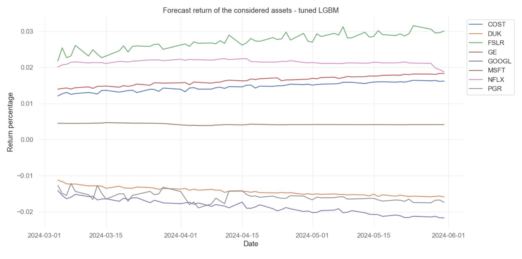
Figure 3: Forecast return of the individual assets from hyperparameter-tuned LightGBM

Figure 3 displays the predicted compounded return percentages for all assets from March to June 2024. The lines do not show extreme volatility, which suggests the model predicts a stable market or smoothes out the extreme fluctuations. Moreover, the trends of each line remain in the same direction, reflecting consistent predictive performance. However, it might also imply that the LightGBM could be oversimplifying the dynamic market movement (See Figure 4).

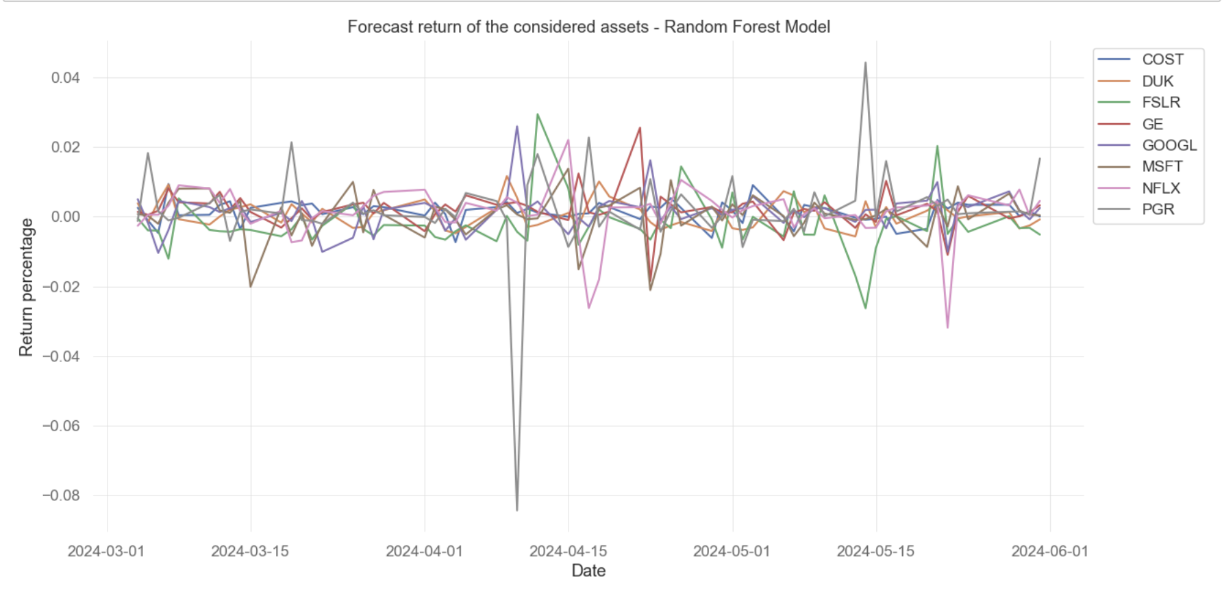
Figure 4: Forecast return of the individual assets from the optimized Random Forest model

The Random Forest model exhibits an RMSE of 0.019581, indicating a relatively lower average error compared to the LightGBM. The low RMSE value suggests that the Random Forest model has performed quite effectively in predicting the returns of assets. The forecasted compounded return predicted by the optimized Random Forest model, from March to June 2024, is represented in Figure 4. The plot exhibits significant fluctuation, with all asset lines illustrating peaks and troughs. It implies that the RF model is sensitive to volatile market movement and can capture short-term shifts in asset performance.

3.2. Efficient Frontier and Optimal Weights

3.2.1. Light Gradient Boosting Model

By numerously performing Monte Carlo simulations, a significant number of portfolios are generated based on random weights and forecast returns predicted by the LightGBM model (See Figure 5).

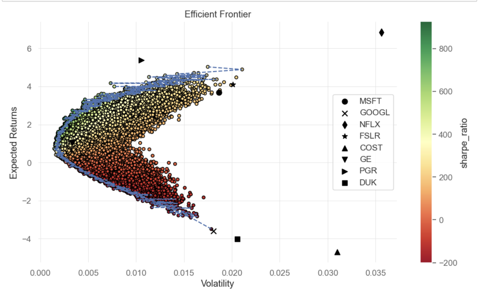
Figure 5: Efficient Frontier - LightGBM model

Evaluated by expected return and volatility, Figure 5 displays the portfolios by points in a scatter plot format. The Efficient Frontier is highlighted by a blue dotted line, delineating the portfolio combinations that achieve the maximized expected gains for defined volatility amount or the minimal volatility for certain expected rewards. Figure 6 showcases the Maximum Sharpe Ratio portfolio identified by the star symbol and the Minimum Volatility portfolio denoted by a plus symbol.

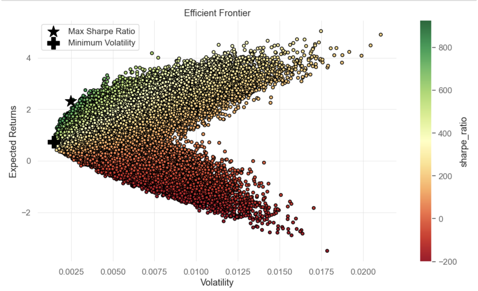
Figure 6: Maximum Sharpe Ratio and Min Volatility Portfolios based on predicted return of LightGBM model

The optimal weights distributed to each asset in the two optimal portfolios are shown in the following Table 3:

Table 3: Weights allocated to each asset in the optimized portfolios based on the forecast return of the LightGBM model

3.2.2. Random Forest Model

By implementing the Monte Carlo Simulation and constructing numerous portfolios from multiplying random weights and forecast results of the Random Forest Model, an Efficient Frontier is plotted in Figure 7.

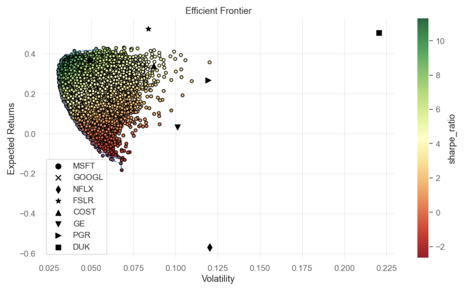
Figure 7: Efficient Frontier - Random Forest model

Figure 8 exhibits the locations of optimal portfolios lying on the Efficient portfolio, denoted by the star sign and the plus sign. Related weights are shown in the following Table 4.

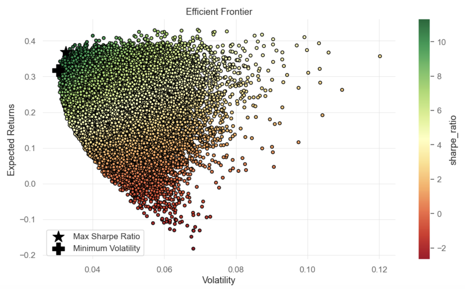
Figure 8: Maximum Sharpe Ratio and Min Volatility Portfolios based on predicted return of Random Forest model

Table 4: Weights allocated to each asset in the optimal portfolios based on the forecast return of Random Forest model

3.3. Backtesting Results

To evaluate the performance of optimal weights in real-life scenarios, portfolios are constructed by applying these weights to actual historical compounded returns, from March to June 2024. The performance of these portfolios is then assessed by computing key metrics, including return, volatility, and the Sharpe Ratio. These measurements provide a comprehensive view of portfolio performance and allow for a detailed comparison against other strategies or benchmarks.

The backtesting results for portfolios optimized using LightGBM and Random Forest models indicate significant performance differences when compared to the S&P 500 benchmark.

3.3.1. Light Gradient Boosting Machine

For the LightGBM model, the Maximum Sharpe Ratio portfolio delivered a remarkable cumulative return of 24.35% with a high annual volatility of 19.1%, significantly outperforming the market, represented by the S&P 500 index, which exhibits a cumulative return of only 2.7% with volatility of 11.2%. Demonstrating superior risk-adjusted performance, the Sharpe Ratio optimized portfolio stands at 4.66, markedly higher than the S&P 500 index’s ratio of 1.02. The Minimum Volatility portfolio based on the LightGBM model presents an even higher return at 28.26% with a slightly increased volatility of 20.7%. Both portfolios surpass the market index in cumulative return and Sharpe Ratio. In comparison, although the annual volatility metrics of both optimized portfolios are markedly above the market’s volatility of 11.2%, it is noticeable that the S&P 500 experienced a higher maximum drawdown of -5.5%, compared to the optimized portfolios. Additionally, while the Minimum Volatility Portfolio is supposed to deliver minimized volatility at a specified level of return in theory, it exhibits slightly higher volatility with a more rewarding cumulative return compared to the Maximum Sharpe Ratio portfolio (See Table 5).

Table 5: Performance metrics of portfolios

3.3.2. Random Forest Model

For the Random Forest model, Table 5 and Table 6 exhibit that all portfolios generated by optimal weights outperform the market performance. The Maximum Sharpe Ratio Portfolio produces an extraordinary cumulative return of 22.52% with a volatility of 18.7%, which surpasses the return of the S&P 500. Meanwhile, it yields a Sharpe Ratio of 4.44, reflecting its effectiveness in providing higher risk-adjusted returns relative to benchmark’s ratio of 1.02. The Minimum Volatility Portfolio also shows a more profitable profile with a cumulative return of 19.09% and a Sharpe Ratio of 4.21. The optimized portfolios undertake annual volatility of around 17% and 18.7%.

Table 6: Performance metrics of portfolios

Based on these results, one could observe the following:

Both the LightGBM and Random Forest models generate portfolios that substantially exceed the performance of the S&P 500 with significantly higher cumulative returns and Sharpe Ratios. It manifests the effectiveness of using machine learning models for portfolio optimization. Both models also demonstrate lower maximum drawdowns than the S&P 500, suggesting that the diversification of portfolio effectively reduces the risk exposure. The Random Forest model shows lower RMSE, which usually indicates greater prediction accuracy. Nevertheless, both its Maximum Sharpe Ratio and Minimum Volatility portfolios deliver lower cumulative returns and lower Sharpe Ratios compared to those from the LightGBM model. While both models show similar volatility levels, portfolios from the Random Forest model tended to have slightly lower returns than those from the LightGBM model. Despite capturing less market dynamic in the aspect of forecast return, the LightGBM’s optimized portfolio exhibits a more remarkable cumulative return and Sharpe Ratios, while maintaining similar levels of volatility. It underscores LightGBM’s superior performance in optimizing risk-adjusted returns.

4. Conclusion

This study investigates the integration of machine learning-based forecast models with portfolio optimization techniques, aiming to identify the optimal asset allocation and introduce a novel approach of investment strategy. Taking historical compounded returns in three quarters as the training set, Light Gradient Boosting Machine and Random Forest models are employed to forecast the daily return of next quarter with a rolling window approach, which ensures the robustness of prediction. On the basis of Mean-Variance Portfolio theory, optimized portfolios are determined by performing Monte Carlo simulations. The strategy of weights allocation is validated by simulating the performance in real-life scenarios backed by actual historical return.

The empirical results manifest that Maximum Sharpe Ratio portfolios and Minimum Volatility portfolios of both models significantly outperform the S&P 500 index with significantly higher cumulative returns and Sharpe Ratios. This confirms the substantial potential of combining machine learning model and portfolio optimization in investment strategy. Notably, despite similar volatility levels and slightly lower predictive accuracy indicated by RMSE, the LightGBM model excels the Random Forest model in achieving higher returns and Sharpe Ratios, indicating a more robust performance in optimizing risk-adjusted return.

These findings highlight the practical utility of machine learning techniques in managing portfolios, substantiating the unexploited potential. The success of these portfolios in outperforming benchmark index presents a compelling vision for investors in contemporary investment strategies. Backtesting with real-time data enhances the reliability and practical applicability in the live trading environments. Future research could leverage advanced machine learning models and incorporate broader economic indicators to refine the forecasting accuracy. Additionally, exploring the relationship between predictive accuracy and portfolio performance in the market could further bolster the efficacy of data-driven investment strategies.

References

[1]. Chen, Y., Zhao, X., & Yuan, J. (2022). Swarm intelligence algorithms for portfolio optimization problems: Overview and recent advances. Mobile Information Systems, 2022, 1–15.
[2]. Chen, W., Zhang, H., Mehlawat, M. K., & Jia, L. (2021). Mean–variance portfolio optimization using machine learning-based stock price prediction. Applied Soft Computing, 100, 106943.
[3]. Markowitz, H. M. (1959b). Introduction (Ser. Efficient Diversification of Investments, pp. 3–7). Yale University Press. Retrieved from http://www.jstor.org/stable/j.ctt1bh4c8h.5.
[4]. Kalayci, C. B., Ertenlice, O., & Akbay, M. A. (2019). A comprehensive review of deterministic models and applications for mean-variance portfolio optimization. Expert Systems with Applications, 125, 345–368.
[5]. Ban, G.-Y., El Karoui, N., & Lim, A. E. (2018). Machine learning and portfolio optimization. Management Science, 64(3), 1136–1154.
[6]. Lee, Y., Kim, M. J., Kim, J. H., Jang, J. R., & Chang Kim, W. (2019). Sparse and robust portfolio selection via semi-definite relaxation. Journal of the Operational Research Society, 71(5), 687–699.
[7]. Zhang, Y., Li, X., & Guo, S. (2017). Portfolio selection problems with Markowitz’s mean–variance framework: A review of literature. Fuzzy Optimization and Decision Making, 17(2), 125–158.
[8]. Bartram, S. M., Branke, J., Rossi, G. D., & Motahari, M. (2021). Machine Learning for Active Portfolio Management. The Journal of Financial Data Science, 3(3), 9–30.
[9]. Yang, F., Chen, Z., Li, J., & Tang, L. (2019). A novel hybrid stock selection method with stock prediction. Applied Soft Computing, 80, 820–831.
[10]. Qiao, R., Chen, W., & Qiao, Y. (2022). Prediction of stock return by LSTM Neural Network. Applied Artificial Intelligence, 36(1).
[11]. Li, J. (2022). The comparison of LSTM, LGBM, and CNN in stock volatility prediction. Proceedings of the 2022 7th International Conference on Financial Innovation and Economic Development (ICFIED 2022).
[12]. Hartanto, A. D., Nur Kholik, Y., & Pristyanto, Y. (2023). Stock price time series data forecasting using the Light Gradient Boosting Machine (lightgbm) model. JOIV: International Journal on Informatics Visualization, 7(4), 2270.
[13]. Li, F., Zhang, L., Chen, B., Gao, D., Cheng, Y., Zhang, X., Yang, Y., Gao, K., Huang, Z., & Peng, J. (2018). A light gradient boosting machine for remainning useful life estimation of aircraft engines. 2018 21st International Conference on Intelligent Transportation Systems (ITSC).
[14]. Basak, S., Kar, S., Saha, S., Khaidem, L., & Dey, S. R. (2019). Predicting the direction of stock market prices using tree-based classifiers. The North American Journal of Economics and Finance, 47, 552–567.
Cite this article
Zhang,Y. (2024). Integrating Forecasting and Mean-Variance Portfolio Optimization: A Machine Learning Approach. Advances in Economics, Management and Political Sciences,90,157-168.
Data availability
The datasets used and/or analyzed during the current study will be available from the authors upon reasonable request.
Disclaimer/Publisher's Note
The statements, opinions and data contained in all publications are solely those of the individual author(s) and contributor(s) and not of EWA Publishing and/or the editor(s). EWA Publishing and/or the editor(s) disclaim responsibility for any injury to people or property resulting from any ideas, methods, instructions or products referred to in the content.
About volume
Volume title: Proceedings of the 3rd International Conference on Financial Technology and Business Analysis
© 2024 by the author(s). Licensee EWA Publishing, Oxford, UK. This article is an open access article distributed under the terms and
conditions of the Creative Commons Attribution (CC BY) license. Authors who
publish this series agree to the following terms:
1. Authors retain copyright and grant the series right of first publication with the work simultaneously licensed under a Creative Commons
Attribution License that allows others to share the work with an acknowledgment of the work's authorship and initial publication in this
series.
2. Authors are able to enter into separate, additional contractual arrangements for the non-exclusive distribution of the series's published
version of the work (e.g., post it to an institutional repository or publish it in a book), with an acknowledgment of its initial
publication in this series.
3. Authors are permitted and encouraged to post their work online (e.g., in institutional repositories or on their website) prior to and
during the submission process, as it can lead to productive exchanges, as well as earlier and greater citation of published work (See
Open access policy for details).