1. Introduction

Market risk refers to the risk of financial losses due to adverse changes in stock prices, interest rates, etc. This issue is not only a core issue of concern to investors and financial institutions, but also an important consideration for regulators when formulating policies. The volatility of market risk may increase the instability of the financial system and even trigger an economic recession in extreme cases. Furthermore, the risk spillover effect across different markets plays a significant role in investment decisions and asset allocation optimization. A deeper understanding of these dynamic mechanisms is essential for enhancing risk management in financial markets, enabling more precise risk identification and improved mitigation strategies [1].

2. Literature Review

Value at Risk (VaR) is a fundamental metric for assessing financial market risk. This section presents a review of the literature on VaR, tracing the development of its widely used computational approaches and their practical applications.

The Historical Simulation method estimates future risk by relying on past market data. Hendricks illustrated that this approach effectively captures stock market risk across various periods; however, its accuracy is heavily influenced by the length of the historical data window used in the analysis [2]. Escanciano and Pei further examined its applicability in emerging markets, observing that its effectiveness declines during periods of heightened market volatility. They proposed that integrating historical simulation with other techniques could improve the precision of VaR estimates [3].

The Monte Carlo simulation method utilizes computational simulations and random sampling techniques to estimate VaR. Pasieczna’s research demonstrated that this approach is particularly effective in capturing risks in highly volatile markets. Increasing the number of simulation paths has been shown to enhance the precision of VaR estimates significantly [4]. Moreover, empirical studies suggest that the Monte Carlo method is especially advantageous for complex asset portfolios, particularly those containing highly nonlinear financial instruments [5].

The Variance-Covariance method, in contrast, estimates VaR based on the assumption that asset returns follow a normal distribution. Hull and White observed that while this approach yields reliable results under stable market conditions, its accuracy deteriorates markedly during periods of financial turbulence [6]. Jorion’s empirical analysis of the foreign exchange market further underscored the method’s limitations, emphasizing its inability to adequately capture non-normal return distributions and its strong dependence on restrictive statistical assumptions [7].

Given the inherent limitations of individual VaR estimation methods, researchers have increasingly explored the benefits of combining multiple approaches. McNeil and Frey, in their study on financial derivatives, found that while the Monte Carlo simulation method tends to perform better in highly volatile market conditions, it comes with significantly higher computational demands [8]. Pérignon and Smith further argued that integrating different methods can improve the accuracy of VaR estimates, particularly during periods of heightened market uncertainty [9]. Ultimately, selecting an appropriate VaR calculation technique—or employing a combination of methods—is essential for strengthening risk management practices.

3. Methodology

This section applies Historical simulation, Monte Carlo simulation, and the Variance-Covariance method to evaluate the Nasdaq Index's market risk. Each method has distinct features in estimating losses, relies on different assumptions, and varies in computational complexity.

3.1. Return and Loss

In finance, a return measures the profit or loss of an investment over a given period, typically represented as a percentage of the initial value. Conversely, a loss refers to a negative return, indicating a decline in portfolio value.

\( R=\frac{{V_{T}}-{V_{0}}}{{V_{0}}} \) (1)

\( Loss=- R \) (2)

Where \( {V_{0}} \) is the initial value of portfolio. \( R \) is the return while \( Loss \) stands for the loss of portfolio [10].

3.2. Value at Risk (VaR)

VaR quantifies the potential loss of a portfolio within a given period, calculated at a predetermined confidence level. It offers a clear measure of the maximum expected loss under normal market conditions.

\( Va{R_{α}}(T)=inf{\lbrace x∈R:P(Loss \gt x)\rbrace }≤1-α \) (3)

This formula implies that VaR is the smallest value \( x \) such that the probability of experiencing a loss greater than \( x \) is no more than \( 1-α \) .

3.3. Historical Simulation Method

The Historical simulation method estimates VaR by ordering historical returns and identifying losses at a given confidence level. Unlike parametric approaches, it derives estimates directly from historical data without assuming a specific return distribution.

\( Va{R_{α,HS}}=-Q({R_{t}},1-α) \) (4)

Where \( α \) represents the confidence level, \( {R_{t}} \) denotes the set of historical returns and \( Q({R_{t}},1-α) \) is the \( (1-α) \) - quantile of the return.

3.4. Monte Carlo Simulation Method

The Monte Carlo simulation method uses a probabilistic model to simulate numerous possible future return scenarios for VaR estimation. This approach effectively captures extreme market movements and models complex nonlinear dependencies. The calculation is given by

\( Va{R_{α,MC}}=-Q({R_{sim}}(t),1-α) \) (5)

Where \( α \) represents the confidence level, \( {R_{sim}}(t) \) represents the simulated returns and \( Q({R_{sim}}(t),1-α) \) is the \( (1-α) \) - quantile of the simulated return distribution.

3.5. Variance-Covariance Method

The Variance-Covariance method calculates VaR under the assumption that returns follow a normal distribution, using the mean and standard deviation. Its computational efficiency and simplicity make it widely applied in practice.

\( Va{R_{α,VC}}={Z_{α}}\cdot σ-μ \) (6)

Where ​ \( {Z_{α}} \) is the critical value from the standard normal distribution with the confidence level \( α \) and portfolio's mean return is \( μ \) .

4. Analysis and Discussion

4.1. Descriptive Statistics

This part provides an overview of the adjusted closing prices of the Nasdaq Index and its daily returns from 2015 to 2024. Daily returns are calculated as percentage changes from the adjusted closing prices of adjacent trading days. This analysis provides a data basis for different methods to calculate VaR.

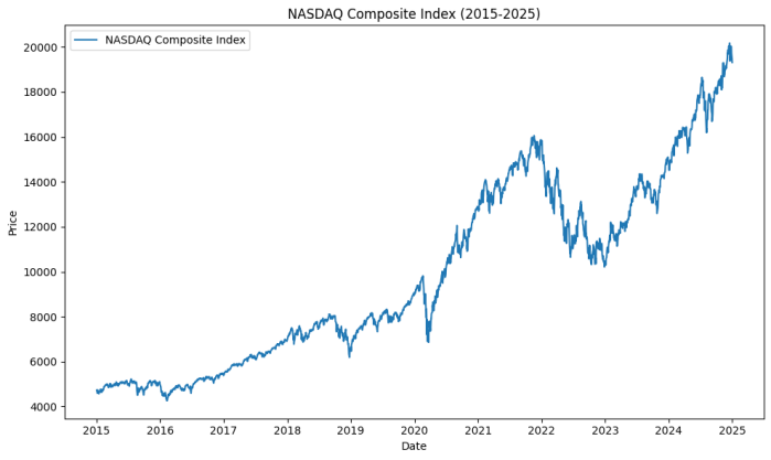
Figure 1: NASDAQ Composite Index (2015-2025)

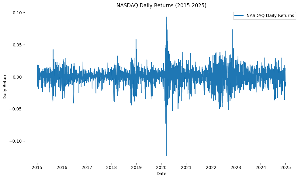
Figure 2: NASDAQ Composite Index Daily Returns (2015-2025)

These two figures reflect the overall growth trend of the NASDAQ Composite Index and the fluctuation of daily returns. The following descriptive statistical indicators, such as the mean and median of daily returns, help analyze the distribution characteristics of the data and reveal the key characteristics of market fluctuations.

Table 1: Descriptive statistical indicators

4.2. Historical Simulation VaR

\( Va{R_{0.95, HS}}=-Q({R_{t}}, 0.05) \) (7)

\( Va{R_{0.99, HS}}=-Q({R_{t}}, 0.01) \) (8)

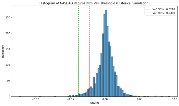
Figure 3: Historical Simulation of NASDAQ Returns with VaR Threshold (95% & 99%)

As can be seen from Figure 3, when the historical simulation method is applied, the NASDQ Composite Index falls by more than 2.19% on 5% of trading days and by more than 3.80% on 1% of trading days.

4.3. Monte Carlo Simulation VaR

When performing a Monte Carlo simulation of the NASDAQ Composite Index, the model first assumes that returns follow a normal distribution and uses the historical mean and standard deviation as model parameters. Then, the 1-day VaR is estimated at 95% and 99% confidence levels by generating 10,000 simulated return paths.

\( Va{R_{0.95, MC}}=-Q({R_{sim}}(t),0.05) \) (9)

\( Va{R_{0.99, MC}}=-Q({R_{sim}}(t),0.01) \) (10)

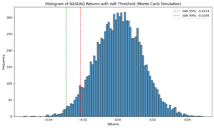
Figure 4: Monte Carlo Simulation of NASDAQ Returns with VaR Threshold (95% & 99%)

Figure 4 shows that the simulated return distribution is centered around zero and exhibits a slight negative skewness, which indicates that negative returns occur slightly more frequently or more dramatically than positive returns. Based on the simulated data, the VaR threshold is -0.0216, which means that there is a 5% probability that the Nasdaq Composite Index will lose more than 2.16% on any given day.

4.4. Variance-Covariance VaR

\( Va{R_{0.95,VC}}={Z_{0.05}}\cdot σ-μ \) (11)

\( Va{R_{0.99,VC}}={Z_{0.01}}\cdot σ-μ \) (12)

where \( μ \) is the mean return, \( σ \) is the standard deviation of returns, and \( {Z_{0.05}} \) ​ and \( {Z_{0.01}} \) are the critical values from the standard normal distribution corresponding to the 95% & 99% confidence level.

Figure 5: Variance-Covariance Simulation of NASDAQ Returns with VaR Threshold (95% & 99%)

As shown in Figure 5, the histogram illustrates that the return distribution is roughly symmetric around the mean, consistent with the normal distribution assumption. The 5th percentile of the VaR threshold is marked by the red dashed line at -0.0215, indicating that there is a 5% probability that the Nasdaq Composite Index will lose more than 2.15% on any given day. Similarly, there is a 1% probability that the loss will exceed 3.07%.

4.5. Comparison of Returns and VaR for Different Models

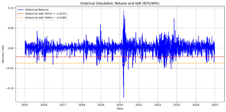
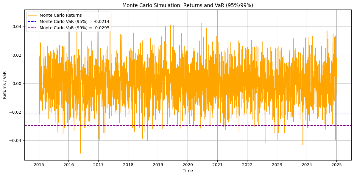
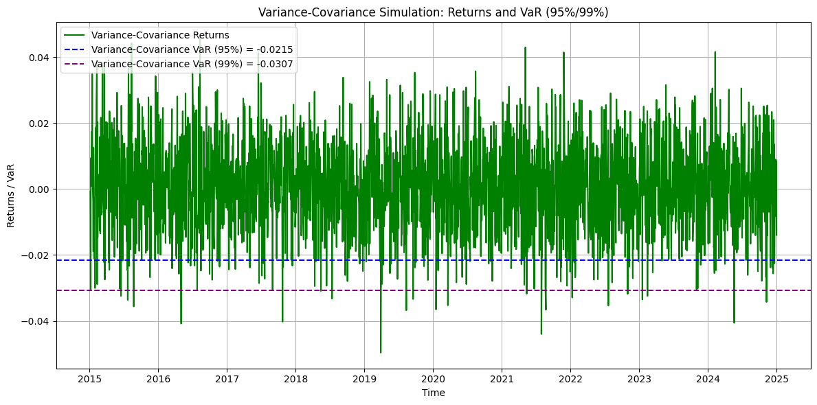
Figure 6: Comparison of Returns and VaR at 95% & 99% for Different Methods

The close proximity of the VaR thresholds indicates consistent risk estimation across methods, but slight differences highlight their distinct approaches.

Table 2: VaR (95% & 99%) for Different Mothods

From Table 2, the VaR estimates of the three methods at 95% and 99% confidence levels are relatively close. However, at the 99% confidence level, the risk values given by the Monte Carlo simulation method and the variance-covariance method are slightly higher than those of the historical simulation method.

Through the above calculations and comparative analysis, the advantages and disadvantages of different VaR methods can be seen. The historical simulation method does not need to make assumptions about the distribution of returns and estimates risks directly based on historical data. However, this method relies on the assumption that "past market behavior can reflect future risks", so it has poor adaptability when dealing with unknown extreme events in the future. The Monte Carlo simulation method provides a more flexible way to assess risk and can simulate a variety of possible market scenarios. However, the effectiveness of this method depends on model assumptions, such as the normal distribution of returns may deviate from the actual situation. If the actual return distribution deviates significantly, the VaR estimate may not accurately reflect the potential risk.

Moreover, its high computational complexity makes large-scale simulations costly, potentially limiting its practicality. The Variance-Covariance method is widely used for its efficiency; however, its reliance on the normality assumption often leads to an underestimation of tail risk. In times of extreme market volatility, such as financial crises, it may fail to capture severe loss risks accurately, thus reducing the reliability of risk management decisions [11].

5. Conclusion

This study compares three VaR calculation methods in the stock market. Results indicate that at a 95% confidence level, VaR estimates across methods are similar. However, at a 99% confidence level, the historical simulation method produces lower VaR estimates than the Monte Carlo simulation and variance-covariance methods. As it directly relies on historical data, the historical simulation method is computationally simple and easy to implement, though it may underestimate risk during extreme market fluctuations. Monte Carlo simulation is more responsive to extreme events, offering a more comprehensive risk evaluation. The variance-covariance method is computationally efficient but depends on the normality assumption, which can lead to underestimating tail risk and extreme market volatility.

Traditional VaR models are typically based on linear assumptions, potentially introducing estimation biases in nonlinear market settings. In contrast, machine learning methods can accommodate high-dimensional data and capture complex nonlinear relationships, improving risk prediction accuracy [12]. This study primarily examines investment risk in a single market, and traditional VaR models may not sufficiently capture risks in cross-asset and cross-market portfolios. Future research should further investigate market volatility and risk transmission mechanisms to enhance portfolio risk management strategies [13,14].

References

[1]. Bouri, E., Lei, X., Jalkh, N., Xu, Y., & Zhang, H. (2021). Spillovers in higher moments and jumps across US stock and strategic commodity markets. Resources Policy, 72, 102060.
[2]. Hendricks, D. (1996). Evaluation of value-at-risk models using historical data. Economic policy review, 2(1).
[3]. Escanciano, J. C., & Pei, P. (2012). Pitfalls in backtesting historical simulation VaR models. Journal of Banking & Finance, 36(8), 2233-2244.
[4]. Pasieczna, A. H. (2021). Model Risk of VaR and ES Using Monte Carlo: Study on Financial Institutions from Paris and Frankfurt Stock Exchanges. In Contemporary Trends and Challenges in Finance: Proceedings from the 6th Wroclaw International Conference in Finance (pp. 75-85). Springer International Publishing.
[5]. Abudurexiti, N., He, K., Hu, D., Rachev, S. T., Sayit, H., & Sun, R. (2024). Portfolio analysis with mean-CVaR and mean-CVaR-skewness criteria based on mean–variance mixture models. Annals of Operations Research, 336(1), 945-966.
[6]. Hull, J., & White, A. (1998). Value at risk when daily changes in market variables are not normally distributed. Journal of derivatives, 5, 9-19.
[7]. Jorion, P. (2007). Value at risk: the new benchmark for managing financial risk. McGraw-Hill.Acerbi, C., &
[8]. McNeil, A. J., & Frey, R. (2000). Estimation of tail-related risk measures for heteroscedastic financial time series: an extreme value approach. Journal of empirical finance, 7(3-4), 271-300.
[9]. Pérignon, C., & Smith, D. R. (2010). The level and quality of Value-at-Risk disclosure by commercial banks. Journal of Banking & Finance, 34(2), 362-377.
[10]. Darmawan, M. R., & Widyono, F. A. P. (2024). Comparative Analysis: Value at Risk (VaR) with Parametric Method, Monte Carlo Simulation, and Historical Simulation of Mining Companies in Indonesia. International Journal of Quantitative Research and Modeling, 5(4).
[11]. Bianchi, M. L., Tassinari, G. L., & Fabozzi, F. J. (2023). Fat and Heavy Tails in Asset Management. Journal of Portfolio Management, 49(7).
[12]. Pala, S. K. Role and Importance of Predictive Analytics in Financial Market Risk Assessment. International Journal of Enhanced Research in Management & Computer Applications ISSN, 2319-7463.
[13]. Liu, X., Shehzad, K., Kocak, E., & Zaman, U. (2022). Dynamic correlations and portfolio implications across stock and commodity markets before and during the COVID-19 era: A key role of gold. Resources Policy, 79, 102985.
[14]. Mahaputra, M. R., Yandi, A., & Maharani, A. (2023). Calculation of Value At Risk using Historical Simulation, Variance Covariance and Monte Carlo Simulation Methods. Siber International Journal of Digital Business (SIJDB), 1(1), 1-8.
Cite this article
Xie,Y. (2025). Historical Simulation, Variance-Covariance and Monte Carlo Simulation Methods for Market Risk Assessment: From NASDAQ Index 2015-2024. Advances in Economics, Management and Political Sciences,171,24-31.
Data availability
The datasets used and/or analyzed during the current study will be available from the authors upon reasonable request.
Disclaimer/Publisher's Note
The statements, opinions and data contained in all publications are solely those of the individual author(s) and contributor(s) and not of EWA Publishing and/or the editor(s). EWA Publishing and/or the editor(s) disclaim responsibility for any injury to people or property resulting from any ideas, methods, instructions or products referred to in the content.
About volume
Volume title: Proceedings of the 3rd International Conference on Management Research and Economic Development
© 2024 by the author(s). Licensee EWA Publishing, Oxford, UK. This article is an open access article distributed under the terms and
conditions of the Creative Commons Attribution (CC BY) license. Authors who
publish this series agree to the following terms:
1. Authors retain copyright and grant the series right of first publication with the work simultaneously licensed under a Creative Commons
Attribution License that allows others to share the work with an acknowledgment of the work's authorship and initial publication in this
series.
2. Authors are able to enter into separate, additional contractual arrangements for the non-exclusive distribution of the series's published
version of the work (e.g., post it to an institutional repository or publish it in a book), with an acknowledgment of its initial
publication in this series.
3. Authors are permitted and encouraged to post their work online (e.g., in institutional repositories or on their website) prior to and
during the submission process, as it can lead to productive exchanges, as well as earlier and greater citation of published work (See
Open access policy for details).