1. Introduction

China, with its vast territory and large population, faces significant challenges from climate change, which affects the environment, economy, and social sustainability. Accordingly, this study selects China’s monthly average temperature data from January 1990 to December 2010 as the foundational dataset for analysis and modeling [1]. For temperature time series data exhibiting significant seasonal characteristics, the conventional ARIMA model is insufficient, as it fails to adequately account for seasonal fluctuations, thereby limiting its modeling accuracy and forecasting capability. To more accurately capture and reflect the seasonal patterns present in the data, it is necessary to employ the Seasonal Autoregressive Integrated Moving Average (SARIMA) model, which is better suited for modeling and forecasting seasonal variations in temperature [2]. SARIMA models are particularly suited for modeling temperature due to the strong seasonality inherent in such data [3].

As a vital component of the climate system, temperature exerts a profound influence on the economy, public safety, agricultural production, and ecological sustainability. The occurrence of extreme temperature events often leads to severe disruptions to societal operations, resulting in substantial economic losses and widespread social impacts. For instance, the widespread low-temperature disaster in southern China in 2008 severely impacted daily life and social operations [4]. Both short-term extreme weather events and long-term global warming trends have become unavoidable climate issues for all nations [5]. Accurately analyzing temperature trends and establishing robust forecasting models can help governments and relevant sectors formulate adaptive policies, optimize resource allocation, and enhance their capacity to respond to extreme weather events.

Although global studies on climate change are abundant, they mainly focus on long-term, large-scale trends. In contrast, research applying time series models such as SARIMA to seasonal temperature data remains limited. While the intensified global warming trend is widely accepted in the context of industrialization, the existence of significant short-term increases in average temperature over recent decades still requires empirical validation. As previously mentioned, being able to forecast short-term cold weather events could provide crucial data for decision-making.

Thus, this study uses monthly average temperature data for China from 1990 to 2009 to construct a SARIMA model, aiming to model and forecast temperature trends. Additionally, this study investigates whether a significant warming trend exists over this 20-year period, offering a theoretical foundation for short-term climate research.

This paper first introduces the SARIMA model's advantages and details the role of its parameters. It then provides a transparent description of data preprocessing, partitioning, and model fitting procedures. Finally, the model's forecast values are compared with the test set, and results are presented in detail.

2. Model building

2.1. Model overview

Compared with the ARIMA model, the SARIMA model incorporates seasonal components, making it more accurate for modeling temperature trends and forecasting. Its general form is \( SARIMA(p,d,q){(P,D,Q)_{s}} \) :

\( {Φ_{p}}({B^{s}}){ϕ_{p}}(B){(1-B)^{d}}(1-{B^{s}}{)^{D}}{y_{t}}={Θ_{Q}}({B^{s}}){θ_{q}}(B){ε_{t}}. \) (1)

The parameters \( p \) , \( d \) , \( q \) represent the non-seasonal autoregressive order, differencing order, and moving average order, respectively. P, D, Q represent the seasonal autoregressive order, seasonal differencing order, and seasonal moving average order. The parameter \( s \) is the seasonal period, which is 12 for monthly data in this study.

2.2. Data processing

The dataset consists of China's monthly average temperatures from 1990 to 2009. The data were obtained from the Berkeley Earth dataset hosted on Kaggle, which includes monthly surface temperature records from 1750 onward. After filtering the dataset using SAS, China's monthly temperature data from 1990 to 2009 were used as the training set, while data from 2010 to 2012 formed the test set.

Stationarity was first assessed using the Augmented Dickey-Fuller (ADF) test. Based on the test results, appropriate differencing (both seasonal and non-seasonal) was determined.

Model selection was performed using the arima() function in R, with the Akaike Information Criterion (AIC) as the selection criterion. The function returns the model with the lowest AIC value. After identifying the optimal model, the ACF plot of the residuals was analyzed.

The final model was used to forecast the next 36 months (2010–2012), and predictions were compared with the reserved test dataset. The MAPE was calculated to evaluate forecasting accuracy—a reliable metric for model validation:

\( MAPE=\frac{1}{n}\sum _{i=1}^{n} |\frac{{A_{i}}-{F_{i}}}{{A_{i}}}|×100\%, \) (2)

where A_i is the actual value and F_i is the forecasted value for month \( i \) . MAPE value below 10% typically indicates good forecasting performance [6].

After that, white noise test will be applied on the residual of the final model. If the residuals look like white noise, it means the model has captured the main patterns in the data, and the remaining variation is just random noise [7].

3. Model results

3.1. Preliminary analysis

As shown in Figure 1, China’s monthly average temperature from 1990 to 2009 exhibits clear seasonal patterns—higher in summer and lower in winter. Figure 2 shows the decomposition of the time series, further confirming the seasonal fluctuations. The trend component suggests a downward trend until around 1995, followed by a gradual increase that slows after 2000. Notably, a decline appears again after 2007, possibly linked to the 2008 cold weather event in southern China.

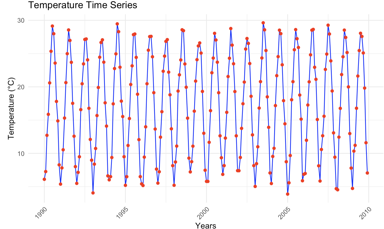
Figure 1: Monthly China temperature from years of 1990 to 2009

The trend component in Figure 2 highlights that although global warming is a long-term reality, short-term average temperature can decline significantly. Accurate prediction of such short-term variations is vital for timely policy responses, especially regarding cold weather events—one of the objectives of this study.

White noise testing on the original data yielded a p-value close to zero, confirming that the series is not white noise and justifying the model building. The ADF test for stationarity produced a p-value of 0.01, which is below the 0.05 threshold. This indicates that the original data are stationary and do not require differencing.

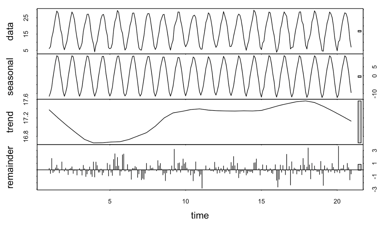
Figure 2: Decomposition of the time series of the original data

Figure 3 presents the ACF plot, revealing strong seasonality, which aligns with expectations: temperatures tend to follow an annual cycle. In summary, the original dataset exhibits characteristics suitable for time series modeling and holds valuable research potential.

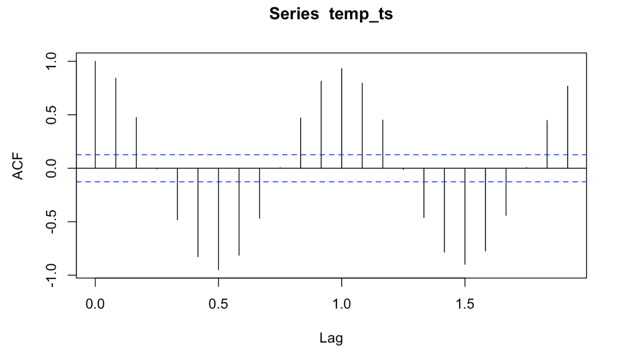
Figure 3: ACF of the original time series

3.2. Final model and validation

Given the seasonality in temperature data, the SARIMA model was adopted. Let R automatically select the model based on the lowest AIC, \( SARIMA(1,0,0){(0,1,2)_{12}} \) with an AIC of 713.04 was chosen.

A Box test on the residuals yielded a p-value of 0.5622, well above 0.05, indicating no significant autocorrelation in the residuals. Thus, the residuals can be regarded as white noise, suggesting the model is appropriate [7].

The forecast() function was used to generate predictions for the next 36 months. The forecasted values and 80% and 90% confidence intervals were extracted and compared with the test data. Figure 4 shows a high level of agreement between predicted and actual values, with the exception of one month in 2011 where the temperature fell outside the 90% confidence interval.

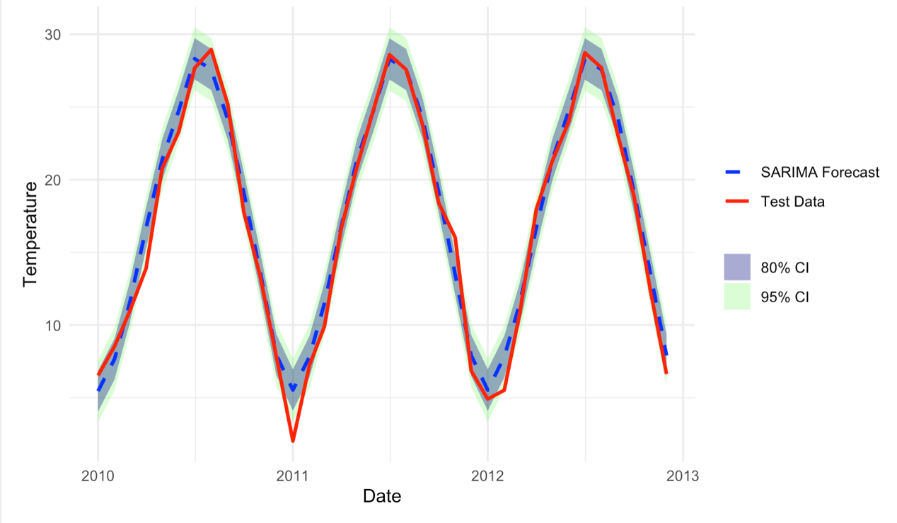
Figure 4: Comparison between the forecast and the real values of the next 36 months

Table 1: The predictions and the actual values for the next 3 years

Table 1 above shows the accurate actual predicted values for test data. Using equation (2), the overall MAPE is 8.37%, which confirms satisfactory predictive performance.

After multiple validations, \( SARIMA(1,0,0){(0,1,2)_{12}} \) demonstrates strong forecasting ability and is selected as the final model. Clearly, the SARIMA model demonstrates significant application value in the study of temperature variation. It helps capture seasonal fluctuations and long-term trends, providing reliable statistical support for climate analysis and forecasting [8].

It is important to note that the dataset presents national average temperatures, potentially overlooking regional variations and extremes across China's vast and diverse geography [9]. Furthermore, relying solely on temperature data fails to encompass the full complexity of climate systems, which are also shaped by factors such as precipitation, wind patterns, and other environmental variables [10].

4. Conclusion

This study analyzed China’s monthly average temperature from 1990 to 2009 using time series methods. The trend component revealed that temperature does not show a consistent upward trend in the short term, and sharp declines may occur. It suggests that short-term warming in China is not yet apparent.

However, this study has limitations. The dataset reflects national average temperatures, which may not represent regional extremes in a geographically diverse country like China. Moreover, temperature alone does not capture the complexity of climate systems, which involve precipitation, wind speed, and other variables. Therefore, the results here serve as a macro-level reference, and specific regions may require tailored analyses.

Using AIC and statistical tests, \( SARIMA(1,0,0){(0,1,2)_{12}} \) was selected as the final model. Validation against actual data confirmed its forecasting accuracy and fulfilled the study’s primary objective. Overall, using the SARIMA model to predict temperature is of great value for people's research and understanding of climate.

In summary, the \( SARIMA(1,0,0){(0,1,2)_{12}} \) model effectively captures the seasonal nature of China's average temperature and provides reliable short-term forecasts. This model holds potential for broader application in temperature prediction and can assist decision-makers in mitigating temperature-related risks and planning for sustainable development.

References

[1]. Yang, Y., Fan, C. and Xiong, H. (2022) A Novel General-Purpose Hybrid Model for Time Series Forecasting: A Novel General-Purpose Hybrid Model for Time Series Forecasting. Applied Intelligence (Dordrecht, Netherlands), 52, 2212-2223.
[2]. Chen, P., Niu, A., Liu, D., Jiang, W. and Ma, B. (2018) Time Series Forecasting of Temperatures using SARIMA: An Example from Nanjing. IOP Conference Series. Materials Science and Engineering, 394, 052024.
[3]. Denton, G. H., Alley, R. B., Comer, G. C. and Broecker, W. S. (2005) The Role of Seasonality in Abrupt Climate Change. Quaternary Science Reviews, 24, 1159-1182.
[4]. Bueh, C., Shi, N. and Xie, Z. (2011) Large‐scale Circulation Anomalies Associated with Persistent Low Temperature Over Southern China in January 2008. Atmospheric Science Letters, 12, 273-280.
[5]. Gillett, N. P., Kirchmeier-Young, M., Ribes, A., Shiogama, H., Hegerl, G. C., Knutti, R., Gastineau, G., John, J. G., L, L., Nazarenko, L., Rosenbloom, N., Seland, Ø., Wu, T., Yukimoto, S. and Ziehn, T. (2021) Constraining Human Contributions to Observed Warming since the Pre-Industrial Period. Nature Climate Change, 11, 207-212.
[6]. Sim, S., Kim, D. and Bae, H. (2023) Correlation Recurrent Units: A Novel Neural Architecture for Improving the Predictive Performance of Time-Series Data. IEEE Transactions on Pattern Analysis and Machine Intelligence, 45, 14266-14283.
[7]. Shao, X. (2011) Testing for White Noise Under Unknown Dependence and its Applications to Diagnostic Checking for Time Series Models. Econometric Theory, 27, 312-343.
[8]. Ray, S., Das, S. S., Mishra, P. and Al Khatib, A. M. G. (2021) Time Series SARIMA Modelling and Forecasting of Monthly Rainfall and Temperature in the South Asian Countries. Earth Systems and Environment, 5, 531-546.
[9]. Jobst, D., Möller, A., and Groß, J. (2024) Time‐series‐based Ensemble Model Output Statistics for Temperature Forecasts Postprocessing. Quarterly Journal of the Royal Meteorological Society, 150, 4838-4855.
[10]. Zhang, K., Huo, X., and Shao, K. (2023) Temperature Time Series Prediction Model Based on Time Series Decomposition and Bi-LSTM Network. Mathematics (Basel), 11, 2060.
Cite this article
Hu,C. (2025). A Study on China's Monthly Temperature Based on the Seasonal Autoregressive Integrated Moving Average. Advances in Economics, Management and Political Sciences,170,60-66.
Data availability
The datasets used and/or analyzed during the current study will be available from the authors upon reasonable request.
Disclaimer/Publisher's Note
The statements, opinions and data contained in all publications are solely those of the individual author(s) and contributor(s) and not of EWA Publishing and/or the editor(s). EWA Publishing and/or the editor(s) disclaim responsibility for any injury to people or property resulting from any ideas, methods, instructions or products referred to in the content.
About volume
Volume title: Proceedings of the 9th International Conference on Economic Management and Green Development
© 2024 by the author(s). Licensee EWA Publishing, Oxford, UK. This article is an open access article distributed under the terms and
conditions of the Creative Commons Attribution (CC BY) license. Authors who
publish this series agree to the following terms:
1. Authors retain copyright and grant the series right of first publication with the work simultaneously licensed under a Creative Commons
Attribution License that allows others to share the work with an acknowledgment of the work's authorship and initial publication in this
series.
2. Authors are able to enter into separate, additional contractual arrangements for the non-exclusive distribution of the series's published
version of the work (e.g., post it to an institutional repository or publish it in a book), with an acknowledgment of its initial
publication in this series.
3. Authors are permitted and encouraged to post their work online (e.g., in institutional repositories or on their website) prior to and
during the submission process, as it can lead to productive exchanges, as well as earlier and greater citation of published work (See
Open access policy for details).