1. Introduction

The principle of a multibeam sounding system involves the use of a set of acoustic transmitters and receivers to emit and receive multiple beams of sound, covering a certain width range. These sound beams propagate underwater, reflect upon encountering the seafloor, and are captured by the receivers. By analyzing the propagation time and angle of the sound waves, the system can accurately calculate the underwater terrain and depth [1]. Over the years, multibeam sounding systems have played a significant role in exploring ocean topography. However, there are some issues regarding measurement accuracy, which have been discussed within the academic community.

Xiangyun Zhou analyzed the measurement accuracy of multibeam sounding systems from the perspective of sound velocity and introduced a sound velocity correction model [2]. Lin Liu summarized various factors causing errors in multibeam sounding and analyzed their mechanisms, proposing corresponding solutions [3]. Jiacheng Yu and his colleagues established a digital bathymetric measurement model for multibeam systems, correcting measurement errors caused by beam angle, carrier attitude effects, and terrain effects [4]. Shengxuan Liu and others suggested using relative error uniformly as the evaluation criterion for line measurement accuracy in multibeam sounding, providing a more objective reflection of the accuracy of multibeam sounding results [5]. Junsen Wang and his team utilized a model to correct edge beam depth data in overlapping regions of adjacent survey lines, effectively reducing measurement errors caused by seafloor terrain [6]. Nong Wang and others evaluated the accuracy of edge beam data in overlapping regions of adjacent survey lines, further establishing an optimization model for correction [7]. Drawing inspiration from the methods of Junsen Wang and Nong Wang, this paper, set against the backdrop of the National College Student Mathematical Modeling Competition, focuses on the measurement errors of edge beams. Considering the impact of overlapping rates of adjacent survey lines on the measurement of edge beams, we conduct an in-depth analysis of the complex relationship between the beam strip coverage width and various parameters in the multibeam sounding system. Multiple optimized deployment schemes for multibeam measurement vessels in various scenarios are proposed. Utilizing differential methods, we calculate the percentage of missed measurements to estimate model accuracy. This study aims to provide more accurate and efficient technical methods for marine measurements, supporting various applications such as marine scientific research, resource exploration, and environmental monitoring.

2. Model Establishment and Solution

2.1. Model Assumptions

Assumption 1: The overlap rate between adjacent strips is not influenced by underwater topography.

Assumption 2: The measurement vessel is treated as a point mass, and factors such as its volume and size are not considered to affect measurement accuracy.

2.2. Establishment of the Coverage Width Model ( \( β=90° \) )

Let the angle between the direction of the survey line and the normal projection of the seafloor slope on the horizontal plane be \( β \) , and let the intersection of the plane perpendicular to the survey line direction and the seafloor slope create a line inclined at an angle \( α \) with the horizontal plane. First, consider the case when \( β=90° \) .

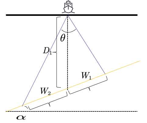
Figure 1. Schematic diagram of coverage width for a single survey vessel

The overlap rate \( η \) between adjacent strips ( \( d \) is the spacing between two adjacent survey lines, and \( W \) is the strip coverage width) is given by:

As shown in Figures 1 and 2, based on geometric relationships and the sine theorem in triangles \( ⊿BOA \) and \( ⊿BOD \) [7], the coverage width W can be expressed as:

Next, calculate the water depth \( z \) , at the center of the survey line (considering the above position as the center), as illustrated in Figure 2:

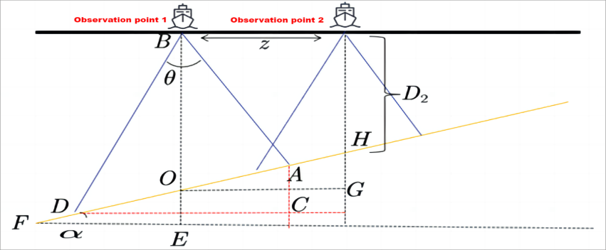
Figure 2. Schematic diagram of overlap rate and coverage width between adjacent survey lines

As shown in Figure 2, \( OG⊥HG \) , \( OG∥FE \) , so \( ∠HOG=∠α \) . In triangle \( ⊿HOG \) , \( OG=α \) , \( HG=ztan{α} \) . \( z \) represents the distance from the survey line to the center point [8], and based on geometric relationships:

Substituting the expression for sea depth \( D(z) \) into equation (2), we obtain [9]:

2.3. Establishment of the Coverage Width Model (Variable \( β \) )

In this paper, the entire sea area is placed within a rectangular prism, aligning the plane containing the survey line with one diagonal face of the prism, as shown in Figure 3. The plane \( UVNB \) corresponds to the plane containing the survey line. The normal projection is known to be parallel to the upper and lower edges of the rectangular sea surface, specifically, the complementary angle to the angle \( β \) formed by the vertical section containing the survey line and the normal projection equals the angle formed by the vertical section containing the survey line and the edge \( BC \) of the rectangular sea surface [10]. Particularly, when \( ∠β=45° \) , the prism is a cube. When \( 0° \lt β \lt 90° \) and \( 270° \lt β \lt 360° \) , the vessel travels towards greater ocean depths.

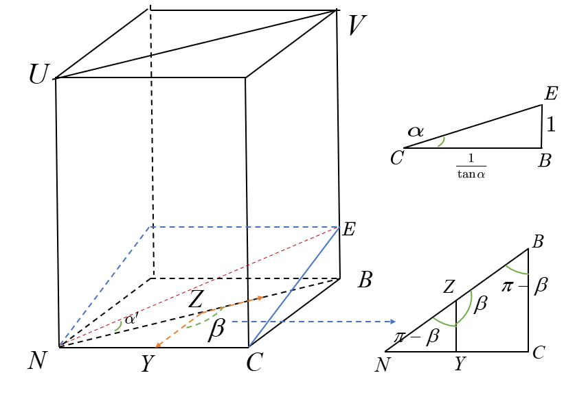
Figure 3. Schematic diagram of a rectangular prism sea area

Assuming the highest point where the seafloor slope intersects with the prism, and the perpendicular line \( BE \) to the sea area ground is 1, the length of the prism’s side \( BC \) is \( 1/tan{α} \) . The slope \( α \prime \) is the angle between the vertical section perpendicular to the sea surface and the intersection line formed by the vertical section and the slope surface, and in \( ⊿NBC \) , the edge \( NB \) can be expressed as \( NB=1/\lbrace tan{α}∙cos{(π-β)}\rbrace \) . In \( ⊿NEB \) , it follows: \( tan{{α^{ \prime }}=-tan{αcos{β}}} \) .

When \( 90° \lt β \lt 270° \) , the vessel travels towards shallower areas. As shown in Figure 3 (right), with the normal projection known to be parallel to the upper and lower edges of the rectangular sea surface, the angle \( β \) formed by the vertical section containing the survey line and the normal projection is equal to the angle formed by the vertical section containing the survey line and the edge \( ND \) of the rectangular sea surface. Similarly, it can be obtained: \( tan{{α^{ \prime }}=tan{αcos{β}}} \) .

Substituting the general functional relationship between \( β \) and slope \( α \prime \) into the established coverage width model (Equation (4)), different coverage width models for various survey line direction angles, or different \( β \) values, can be derived:

Where:

2.4. Genetic Algorithm-Based Survey Line Selection Model

2.4.1. Assumption of No Seafloor Slope in a Certain Sea Area. In this study, Python software is employed to process the bathymetric data obtained from single-beam measurements in the sea area, resulting in the seafloor depth distribution map shown in Figure 4. Deeper colors indicate greater seafloor depths, while lighter colors signify shallower depths.

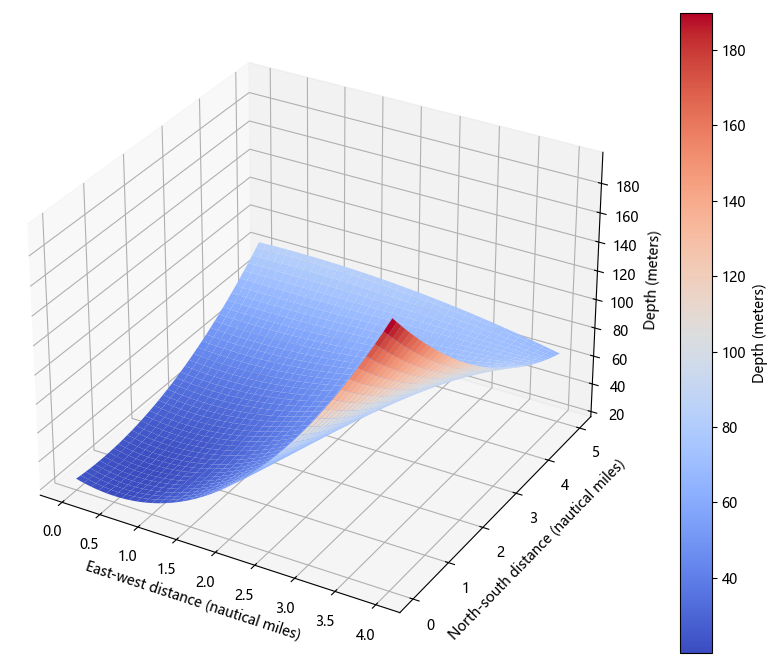
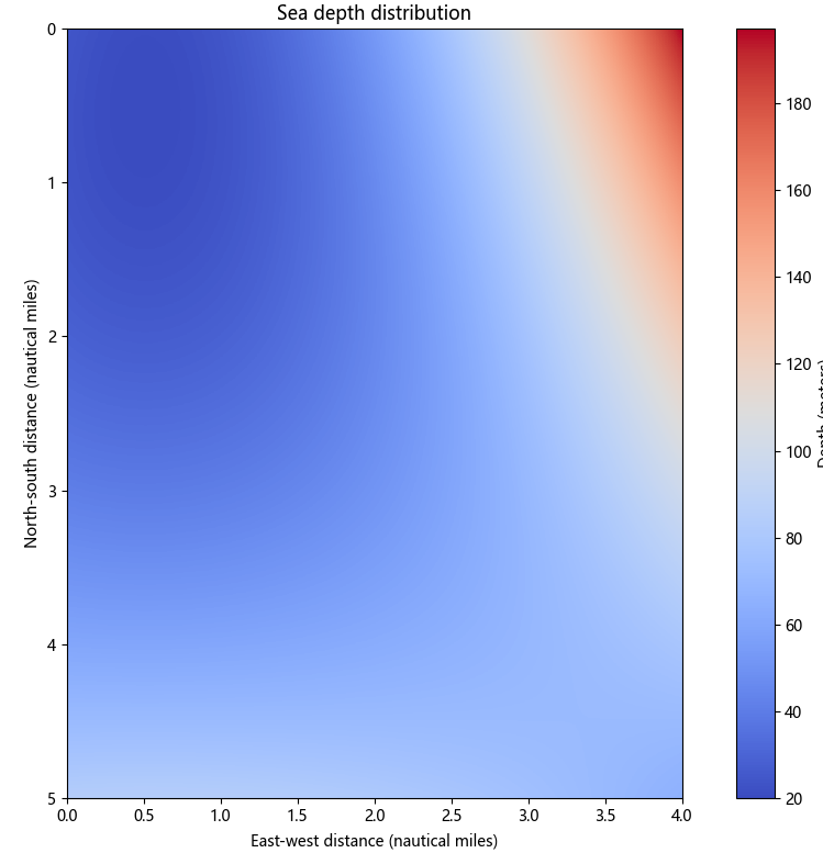
Figure 4. Seafloor depth distribution

Upon analyzing the dataset, it was observed that for every increase of 0.02 nautical miles on both the horizontal and vertical axes, the seawater depth fluctuates within a small range. To simplify the model, it is assumed that the seafloor topography can be approximated as flat within this small range [11].

2.4.2. Determination of the Objective Function. This model can be considered as a single-objective optimization model, with the optimization goal of minimizing the total length of survey lines. The mathematical expression is as follows (where \( n \) is the total number of survey lines):

Since the overlap rate \( η=1-\frac{d}{W}=\frac{W-d}{W} \) , where \( d \) is the effective overlap width, the shortest total length of survey lines can be expressed as the sum of effective overlap widths, as shown below after further simplification of the optimization goal:

2.4.3. Determination of Constraint Conditions. There are two constraint conditions. The first condition aims to cover the entire sea area with the bands formed by scanning along the survey lines as much as possible. To simplify model calculations, it is assumed that the first measurement vessel is positioned at the boundary of the sea area, and the length of the bands formed by scanning along the survey lines is the sum of the effective overlap widths of all survey lines plus the non-overlapping area of the last measurement vessel in the sea area. Here \( \frac{W}{2} \) is approximated as the length of the non−overlapping area of the last measurement vessel in the sea area. The mathematical expression is as follows (where \( ω \) is the east-west width of the rectangular sea area):

The second constraint condition aims to control the overlap rate between adjacent bands to be below 20%, i.e., the minimum overlap rate is 0, and the maximum overlap rate is 20%. Thus:

2.4.4. Summary of the Optimization Model. The final summary of the survey line selection optimization model is as follows:

2.5. Solution of the Survey Line Selection Model

Based on the objective function and constraint conditions mentioned above, a genetic algorithm model is employed for optimization. The genetic algorithm is a type of optimization algorithm inspired by evolutionary principles in biology. The genetic algorithm model estimates the number of survey lines in the layout, and the mean value of \( d \) is implemented for this purpose. The minimum value of \( d \) is the product of \( W \) and the minimum non−coverage rate, and the maximum value of \( d \) is the product of \( W \) and the maximum non-coverage rate. The mathematical expressions are as follows:

Taking the average of these values as the spacing, the estimated number of survey lines can be obtained by dividing the east-west width of the sea area by the spacing. Through Python programming, the estimated number of survey lines is determined to be 37, which is then applied for initializing the population. Subsequently, the genetic algorithm continuously optimizes the results through operations such as crossover and mutation. After 500 iterations, the final survey line layout is obtained as shown below (see Appendix Table 1 for survey line layout coordinates):

Figure 5. Design of survey lines for multi-beam survey vessel

2.6. Solution of the Undetected Area Model

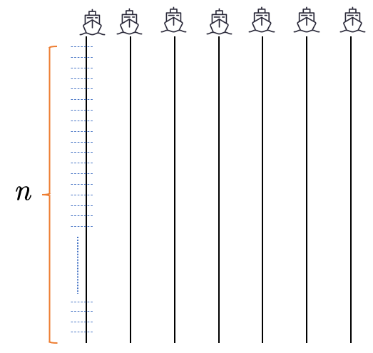
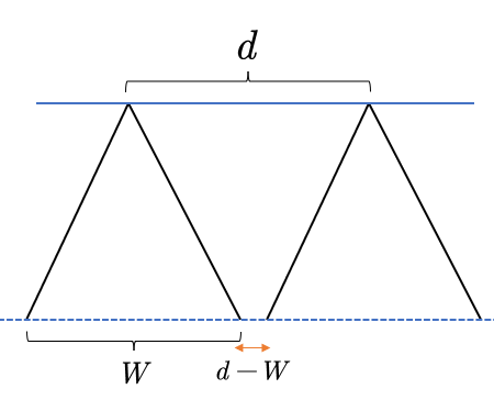
Figure 6. Diagram of leakage between adjacent routes

In the optimized survey line configuration described above, the survey lines are oriented in the north-south direction, and the seawater depth varies at different positions along each survey line. Utilizing the method of differentiation, each survey line is divided into \( n \) points. As \( n→∞ \) , the overlap rate between each point and the corresponding point on the adjacent survey line is calculated. When the overlap rate \( η \lt 0 \) , indicating an undetected region between two survey lines, the length of the undetected region is \( d-W \) , as illustrated in Figure 6. The distance between adjacent points on the same survey line is \( \frac{l}{n} \) , where \( l \) is the length in the north-south direction of the rectangular sea area, and \( l=5NM \) . Iterating through the points with \( η \lt 0 \) , the number of points where the overlap rate is less than 0 is determined. The sum of the areas of these undetected small points gives the total area of the undetected sea region. The formula is expressed as follows ( \( m \) is the total number of undetected points):

Given the constraint condition that the overlap rate exceeds 20%, i.e., \( 1-\frac{d}{W} \gt 0.2 \) , the number of points \( q \) , where the overlap rate exceeds 0.2 is calculated. The total length is \( \frac{5q}{n} \) nautical miles.

The total length of survey lines = Number of side lines × North-south length of sea area. Using Python software for calculation, the results are as follows:

(1) The total length of survey lines is 342,640 meters;

(2) The percentage of the undetected sea area to the total area to be surveyed is approximately 32.774%;

(3) In the overlapping region, the length of the part where the overlap rate exceeds 20% is 35,896.33466 meters. Additionally, the percentage of this part to the total length of survey lines is 10.477%. This confirms the accuracy of the established model.

3. Conclusion

This study successfully applied a genetic algorithm to optimize the layout of multi-beam survey lines, achieving efficient and accurate measurement of seafloor topography. By establishing a nonlinear programming model, this paper optimized the layout of survey lines to maximize coverage of the area to be surveyed while maintaining an overlap rate below 20%. The experimental results demonstrate that the model can significantly reduce measurement errors (approximately 32.774%) and overlap rates (approximately 10.477%), confirming the effectiveness and precision of the model. This approach provides a new means for the field of marine measurements, holding significant importance for applications in marine scientific research, resource exploration, and environmental monitoring.

References

[1]. Wang, F. F., & Ma, Y. (2023). Design and Implementation of Line Deployment System for Multibeam Measurement in Polar Oceans. Marine Information Technology and Application, 38(03), 158-162+186.
[2]. Zhou, X. Y. (2023). Analysis of Errors in Multibeam Sounding Systems and Application of Sound Velocity Correction Models. Longitude and Latitude, 2023(02), 13-16.
[3]. Liu, L. (2023). Causes and Solutions of Distortion in Multibeam Sounding Data. Value Engineering, 42(21), 125-128.
[4]. Yu, J. C., & Xu, X. Q. (2015). Multibeam Sounding Model Based on Attitude and Terrain Effects. Journal of System Simulation, 27(04), 824-829.
[5]. Liu, S. X., Zhang, Y., Ma, J. F., et al. (2016). Discussion on Accuracy Evaluation Method of Multibeam Sounding Results. Marine Surveying and Mapping, 36(05), 36-39.
[6]. Wang, J. S., Jin, S. H., Bian, Z. G., et al. (2023). Correction of Multibeam Sounding Yaw Motion Residuals Using Overlapping Regions of Adjacent Survey Lines. Journal of Ocean Technology, 42(04), 35-42.
[7]. Wang, N., Huang, J., & Rao, T. T. (2023). Line Optimization Model for Multibeam Sounding Systems. Electronic Acoustics Technology, 47(06), 61-64.
[8]. Liang, Y. (2014). Application of Multibeam Measurement Technology in Shallow Seafloor Topography Detection. Modern Surveying and Mapping, 37(02), 19-21.
[9]. Cheng, F., & Hu, N. C. (2016). Research on Optimization Method of Multibeam Measurement Line Deployment. Journal of Ocean Technology, 35(02), 87-91.
[10]. Lin, J. T., Guo, H., & Zhang, X. Y. (2009). Discussion on Several Factors Affecting the Accuracy of Multibeam Measurement. Water Resources and Hydroelectric Engineering, 2009(01), 34-36+40.
[11]. Breaking analysis of solitary waves for the shallow water wave system in fluid dynamics [J]. Duran Serbay, Kaya Doğan. The European Physical Journal Plus.
Cite this article
Li,H.;Li,Y.;Ran,Y.;Wang,Y.;Lan,X. (2024). Optimization model for multibeam sounding line deployment based on genetic algorithm. Theoretical and Natural Science,34,193-200.
Data availability
The datasets used and/or analyzed during the current study will be available from the authors upon reasonable request.
Disclaimer/Publisher's Note
The statements, opinions and data contained in all publications are solely those of the individual author(s) and contributor(s) and not of EWA Publishing and/or the editor(s). EWA Publishing and/or the editor(s) disclaim responsibility for any injury to people or property resulting from any ideas, methods, instructions or products referred to in the content.
About volume
Volume title: Proceedings of the 3rd International Conference on Computing Innovation and Applied Physics
© 2024 by the author(s). Licensee EWA Publishing, Oxford, UK. This article is an open access article distributed under the terms and
conditions of the Creative Commons Attribution (CC BY) license. Authors who
publish this series agree to the following terms:
1. Authors retain copyright and grant the series right of first publication with the work simultaneously licensed under a Creative Commons
Attribution License that allows others to share the work with an acknowledgment of the work's authorship and initial publication in this
series.
2. Authors are able to enter into separate, additional contractual arrangements for the non-exclusive distribution of the series's published
version of the work (e.g., post it to an institutional repository or publish it in a book), with an acknowledgment of its initial
publication in this series.
3. Authors are permitted and encouraged to post their work online (e.g., in institutional repositories or on their website) prior to and
during the submission process, as it can lead to productive exchanges, as well as earlier and greater citation of published work (See
Open access policy for details).