1 Introduction

In the realm of contemporary scientific research, molecular simulation has emerged as a powerful tool for understanding and predicting molecular interactions and their motion under various conditions. Molecular simulation provides scientists with a means to simulate the molecular world, delving deep into how atoms and molecules influence one another in diverse environments, offering valuable insights into various chemical and biological processes [1].

The motion of molecules within a solution plays a pivotal role in many chemical reactions and biological processes, with diffusion being a crucial phenomenon. The diffusion coefficient, often denoted as D, quantitative measurements of the rate at which a diffusion process occurs, which quantifies the random motion of molecules under specific conditions [2]. This random molecular motion is attributed to collisions and thermal movement among molecules, a behavior elucidated by statistical [3]. The random walk of molecules in a thermodynamic equilibrium state leads to the occurrence of diffusion, a phenomenon that holds significant importance in numerous natural phenomena and technological applications. Einstein’s mean square displacement (MSD) method, an integral component of statistical mechanics, further illuminates the calculation of the diffusion coefficient, providing a comprehensive understanding of molecular motion in various environments [4].

The methodology of simulating Brownian motion through computer simulations has been a reliable avenue for investigating the motion of particles [5]. Unlike traditional particle simulations, conducting large-scale simulations poses significant computational challenges [6]. However, the use of Brownian motion simulation programs offers an effective means to streamline computations while maintaining a certain level of accuracy. This paper is focused on employing this research methodology to thoroughly explore the influence of temperature on diffusion coefficients.

In this research, we initiate our exploration by employing a one-dimensional random walk model, a versatile tool for investigating the impact of simulation direction, particle quantity, and simulation duration on the resulting diffusion coefficients [7].

By restricting the simulations to one dimension, we scrutinize the influence of the simulation direction on the computed diffusion coefficients. The choice of direction becomes pivotal, reflecting the particles’ response to an applied force and providing insights into how external factors shape diffusion dynamics.

Furthermore, we address the influence of particle quantity on simulation outcomes. Iterating simulations with the same particle quantity reveals a characteristic normal distribution of results. This statistical approach, rather than a simple averaging method, proves to be a more robust means of extracting meaningful information from multiple simulations. The resulting distribution offers a nuanced perspective, capturing the inherent variability in the system and enhancing the reliability of our simulated results.

Additionally, we investigate the temporal aspect by considering the impact of simulation duration on the observed diffusion coefficients. Short-term simulations may be susceptible to the “cave effect,” where transient fluctuations dominate the results. In contrast, longer simulations tend to stabilize the outcomes, allowing for a more comprehensive understanding of the diffusion process. Recognizing the temporal dynamics contributes to refining the accuracy and reliability of our simulated diffusion coefficients.

In summary, our approach integrates the one-dimensional random walk model to systematically examine the intricate interplay of simulation direction, particle quantity, and simulation duration on the derived diffusion coefficients. This multifaceted exploration lays the groundwork for a comprehensive understanding of the factors influencing molecular diffusion in our simulated systems. With these concepts, this research will focus on the effect of temperature on diffusion.

2 Method

2.1 Method: Einstein’s Relationship for Calculating Diffusion Coefficient (D)[4]

Einstein’s relationship, developed by Albert Einstein in the early 20th century, provides a powerful and fundamental method for calculating the diffusion coefficient (D) in various systems. This relationship is based on the concept of mean square displacement (MSD) and offers valuable insights into the random motion of particles, facilitating a quantitative understanding of their diffusion behavior.

Mathematically, Einstein’s relationship can be expressed as [8]:

\( D=\frac{MSD}{6t}\ \ \ (1) \)

Where:

D represents the diffusion coefficient.

\( MSD(t)= ⟨|r(t)- r(0)|^{2}⟩\ \ \ (2) \)

MSD is the mean square displacement, which characterizes the average squared distance a particle travels from its initial position. t is the time elapsed.

This relationship demonstrates that the diffusion coefficient is directly proportional to the mean square displacement and inversely proportional to both the time elapsed and the dimensionality of the system.

Einstein’s relationship is a cornerstone in the study of diffusion, as it allows for the determination of D from experimental or simulated data involving the motion of particles [8]. By employing this relationship in our study, we can quantitatively evaluate how factors such as time, the number of particles, and directionality influence the diffusion coefficient, providing a rigorous foundation for our research and insights into particle motion in the one-dimensional random walk model.

2.2 One-Dimensional Random Walk Model:

A random walk model is a mathematical concept used to describe a sequence of random steps taken by an entity in a certain space [9]. In this model, the entity’s movement at each step is determined by random factors, making it a stochastic or probabilistic process. In a random walk, the entity’s path unfolds through a series of discrete steps, and the direction of each step is randomly chosen. The randomness in the process reflects the inherent unpredictability associated with each move, creating a dynamic and evolving trajectory for the entity [10]. The random walk model is versatile and finds applications in various fields such as physics, finance, and biology, providing insights into the behavior of dynamic systems influenced by chance [11]. The simplicity of the model makes it a fundamental tool for understanding stochastic processes in diverse contexts.

In this study, we have employed a one-dimensional random walk model to investigate the random motion of particles in one-dimensional space. This model enables us to systematically explore how the following factors influence the simulation results:

Direction: In the model, particles choose to move either left or right at each time step in a random manner. This effectively simulates the random motion of molecules, where changes in direction are stochastic.

Number of Particles: We have the ability to control the quantity of particles in the simulation, thereby studying the influence of different numbers of particles on the results. This allows us to observe how the results change when introducing more or fewer particles in the simulation.

Simulation Time: Time is represented in the model in discrete time steps. We can extend or shorten the total simulation time to investigate the impact of time on the results. This helps us understand how the distribution of particles evolves over time.

By using this model, we are able to systematically study how these key factors in molecular simulations affect the ultimate results. This approach facilitates a deeper understanding of the random motion behavior of molecules in one-dimensional space and provides us with a framework for insights into the results, better explaining the dynamic behavior of molecules under specific conditions.

2.2.1 The influence of direction. In this part, we discuss the behavior of one-dimensional random walk model under the condition of unidirectional movement. Instead of the traditional two-way random walk model, we modify the model to only allow particles to move in the same direction at each time step. With this method, we can model the behavior of particles under external forces or situations where there is a potential energy gradient in a particular direction. We use computer simulations to track the displacement of particles over a fixed period of time and analyze the statistical properties of their displacement to understand the effects of one-way movement on particle behavior.

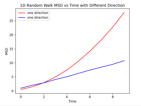
Figure 1. Comparison of MSD of different directions. The blue line is the regular result of MSD change with time. According to Einstein’s Relationship, the blue line can be approximated seen as a linear relationship, which the slope would be six times the diffusion coefficient. The red line is the result when particles could only move towards one direction, which indicates MSD and time have a quadratic function relationship.

2.2.2 The impact of time. Random Walk Simulation Algorithm: The code likely encompasses a random walk simulation algorithm to model the movement of particles over time. This algorithm would generate random steps or movements, mimicking the stochastic nature of particle motion in confined spatial conditions [8].

Calculation of Mean Squared Displacement: Within the code, there is a segment dedicated to calculating the Mean Squared Displacement at each time step. This involves tracking the position of particles over time, computing the squared distance from the initial position, and averaging these squared distances across all particles.

\( MSD(t)= ⟨|r(t)- r(0)|^{2}⟩\ \ \ (3) \)

Dynamic Diffusion Coefficient Calculation: The diffusion coefficient is not a static value but dynamically calculated at each time step. The code likely involves dividing the MSD by a factor related to time (commonly 6 times the time elapsed) to obtain the diffusion coefficient at each time point. [4]

Iterative Simulations for Robust Results: The program may involve running multiple simulations iteratively, each with different random processes or initial conditions. This iterative approach aims to provide statistically robust results, capturing variations in diffusion behavior inherent in stochastic systems.

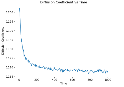
Figure 2. The diffusion coefficient convergence with time. The blue line shows how the diffusion coefficient change with time. At the beginning of the simulation, the diffusion coefficient dropped sharply and eventually oscillating back and forth at a fixed value.

The figure shows a curve of the diffusion coefficient (Y-axis) over the simulation time (X-axis), with special emphasis on the effect of the cave effect. At the beginning of the simulation, the diffusion coefficient dropped sharply, and this change reflect the spatial limitations and nonlinear interactions encountered by the particles at smaller scales, which we call ‘cave effect’ here. With the increase of simulation time, this effect weakens, the particles gradually explore a larger space, and the decline of the diffusion coefficient tends to stabilize. This process may indicate that in the early stages of the simulation, the system is more constrained by initial conditions and local structure, while the diffusion behavior on long time scales is more reflective of macroscopic physical properties. Therefore, in order to ensure that the calculation of the diffusion coefficient can accurately capture the dynamic changes caused by the cave effect, it is recommended to conduct a simulation time long enough to enable the system to reach thermodynamic equilibrium and move beyond the initial nonlinear response phase. This provides guidance on how to time simulations in order to capture and understand the complex behavior of molecular diffusion under confined spatial conditions.

Through numerical simulations, we investigated the relationship between the measured diffusion coefficient and time at different time intervals. Specifically, we conducted multiple random walk simulations to model the diffusion process of particles in one-dimensional space. For each time point, we computed the average Mean Squared Displacement (MSD) from multiple simulations and the corresponding diffusion coefficient. The diffusion coefficient represents the slope of the relationship between mean squared displacement and time, reflecting the average diffusion behavior of particles per unit time.

To better understand the stability of our measurements, we performed multiple simulations at each time point and calculated the standard deviation of the diffusion coefficient [12].

\( s=\sqrt[]{\frac{\sum_{i=1}^{n} (X_{i}-\bar{X})^{2}}{n-1}}\ \ \ (4) \)

By conducting 100 simulations, we obtained the standard deviation at each time point, allowing us to estimate the uncertainty in our measurements. The variation of the standard deviation over time serves as an indicator of the measurement’s stability, helping us assess the reliability of our results.

The trend of the standard deviation over time, shown on the right side of the figure, provides an intuitive understanding of the precision and stability of our measurements. This approach offers a comprehensive and reliable means to evaluate the accuracy of diffusion coefficient measurements, providing robust support for subsequent data interpretation and experimental design.

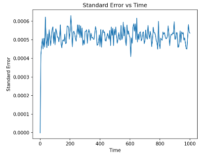
Figure 3. Standard Error convergence with time It shows that the standard error is very low at the first, and then sharply increase with time. Eventually the value oscillates back and forth at a fixed value.

The figure shows how the standard error (Y-axis) changes over simulation time (X-axis) in a one-dimensional random walk simulation. As can be seen from the graph, the standard error drops rapidly in the initial phase and then stabilizes over time. This trend reflects the significant influence of randomness on the estimation of the diffusion coefficient over a short period of time, while the standard error gradually decreases and tends to a constant value over a long period of time due to statistical effects. The fluctuations in the figure show that the estimation of the diffusion coefficient is still affected by random fluctuations even in the long-time simulation. This graph provides us with an intuitive understanding of simulation accuracy and time-scale dependence, highlighting the importance of sufficient simulation time to obtain stable and reliable diffusion data.

2.2.3 The influence from the number of the particles.

Figure 4. Comparison of MSD of different particle numbers This diagram shows the change in the mean square displacement (Y-axis) of 10 particles (blue curve group) and 1000 particles (red curve group) over time (X-axis) in a one-dimensional random walk simulation. Each red curve represents the change in the mean square displacement of a system instance of 10 particles over 1000 time steps, while the blue curve represents a system instance of 1000 particles over the same time step.

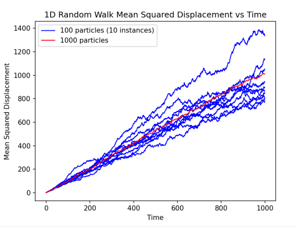
As can be seen from the figure, systems with larger particle numbers show a higher degree of statistical consistency, i.e., the blue curve has less fluctuation, while systems with smaller particle numbers (the red curve) show more fluctuation, indicating that the effect of statistical fluctuations is more significant in smaller systems. These results indicate that increasing the number of particles in the system can effectively reduce random errors, thus providing more stable and reliable predictions of diffusion behavior at the macro scale.

Figure 5. The negative correlation between Standard Error and Numbers of particles. This diagram depicts how the standard error (Y-axis) varies with the number of particles (X-axis) in a one-dimensional random walk simulation. It can be observed that with the increase of the number of particles, the overall trend of the standard error decreases, indicating that more particles help to reduce the random fluctuation and uncertainty of the diffusion coefficient estimation.

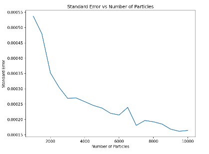
At the beginning, the standard error dropped rapidly, then gradually flattened out, but there were slight fluctuations at some points. These fluctuations may be due to statistical fluctuations in specific particle numbers. The data in the figure shows that when conducting particle diffusion simulations, choosing an appropriate number of particles is crucial to obtain a stable and reliable diffusion coefficient. In addition, the chart hints at potential caving effects to consider when designing experiments and interpreting data, that is, possible nonlinear relationships between particle numbers and simulation results. In order to accurately reflect the diffusion properties of macroscopic systems, simulations on long time scales are recommended when the number of particles is large enough to cover a wide statistical distribution.

From this, we infer that this motion is normally distributed for the same number of particles, and the Shapiro-Wilk method is used to test it [13].

Figure 6. Distribution of Diffusion Coefficient The diagram shows the distribution of Diffusion coefficient for simulating 1000 times. Shapiro-Wilk Test Statistic: 0.99908, P-value: 0.91217.	Figure 7. The verification of normal distribution The Quantile-Quantile Plot of the distribution of Diffusion coefficient. The blue dots are from our data and the red line represents the normal distribution.

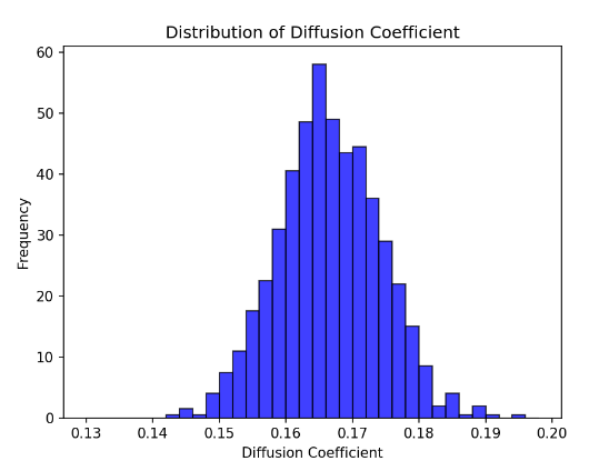
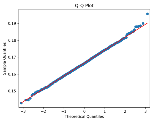
From the result of Shapiro-Wilk method, the P-value is 0.91, which shows that the simulation followed normal distributions. In order to see this relationship further intuitively, we draw the Quantile-Quantile Plot, which shows most of the data is close to the normal distribution [14].

2.3 Brownian motion simulation

Brownian motion, named after the 19th-century botanist Robert Brown who first observed it, is a random motion phenomenon exhibited by particles suspended in a fluid. This seemingly erratic movement is a result of continuous and random collisions with surrounding molecules. In a Brownian motion scenario, the particles experience a constant bombardment from surrounding solvent molecules, leading to abrupt and unpredictable changes in their positions [15]. This motion is a fundamental manifestation of the kinetic nature of matter, providing insights into the dynamic interactions at the molecular level. The mathematical description of Brownian motion involves modeling the particle’s position as a stochastic process, typically described by the Wiener process or the Langevin equation [16]. Brownian motion has played a pivotal role in scientific advancements, contributing to our understanding of diffusion processes, molecular dynamics, and stochastic phenomena.

The differential equation describing Brownian motion, specifically in the overdamped (or strongly damped) regime, can be expressed using the Langevin equation [16]. Overdamped motion typically occurs in situations with significant viscous forces, such as slow movement in a viscous fluid.

The general form of the Langevin equation is [17]:

\( m\frac{dv}{dt}=-γv+\sqrt[]{2γk_{B}T}R(t)\ \ \ (5) \)

m is the mass of the particle,

v is the velocity of the particle,

γ is the viscous damping coefficient,

k_B is the Boltzmann constant,

T is the temperature,

R(t) is a random force obeying a normal distribution.

In the case of overdamped motion, where the viscous damping is large (γ is very large), the acceleration time scale is much smaller than the velocity time scale. This allows us to assume dv/dt​≈0. The Langevin equation then simplifies to:

\( [0=-γv+\sqrt[]{2γk_{B}T}R(t)]\ \ \ (6) \)

Methodology Introduction: Simulating Brownian Motion for Three-Dimensional Trajectory Analysis

In the context of this study, the simulation of Brownian motion serves as a pivotal technique to model the stochastic behavior of particles in a three-dimensional space. Brownian motion, characterized by the random movement of particles suspended in a fluid, is central to understanding various physical phenomena. The employed methodology approximates this intricate process by discretizing time into steps and simulating random displacements at each interval.

The fundamental principle underlying this approach lies in the mathematical representation of Brownian motion as a series of random steps. Each step is determined by a random variable drawn from a normal distribution, capturing the inherent uncertainty in the particle’s trajectory. The variance of these random steps is scaled by the square root of the time interval, aligning with the theoretical underpinnings of Brownian motion [18].

The simulation process unfolds in three dimensions, mirroring the spatial complexity of real-world scenarios. The accumulation of these simulated steps over time generates a trajectory that emulates the unpredictable and continuous nature of Brownian motion. Importantly, the simulation adheres to the physical essence of Brownian motion, where particles experience random forces akin to those exerted by surrounding fluid molecules.

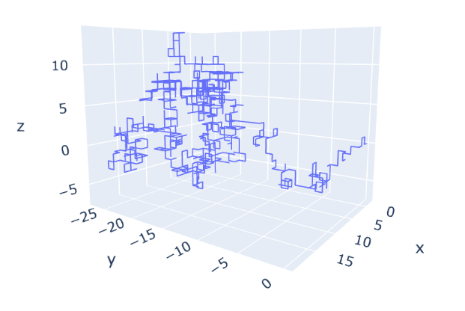
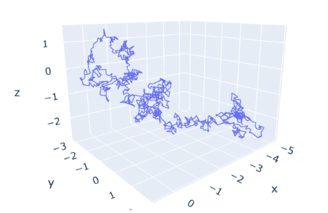
Through the 3-D diagrams of the motion of the single particles in the simulation, we can clearly conclude that this method makes the particle go different directions rather than the original four directions. And the scale of the movement of Brownian simulation is much smaller than that of random walk models.

Figure 8. The routes of a particle in 3-D random walk models. The diagram shows that the range of this route is about 15*25*10. And the angle of rotation is 90 degrees.	Figure 9. The routes of a particle in Brownian motion simulation. The diagram shows that the range of the simulation is about 5*4*4. The angle of rotation is random degrees.

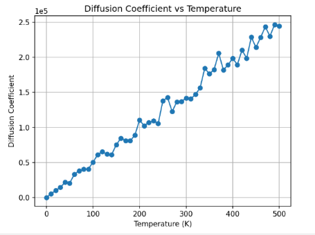
2.4 The effect of temperature on diffusion

With the methods talked before, we can arrive to the final results. Linear regression can be used to analyze the result [19].

Figure 10. Effect of temperature The diagram shows the relationship between temperature and Diffusion coefficient. It seems to be a linear relationship.	Figure 11. Linear relationship verification The diagram shows result the linear regression.

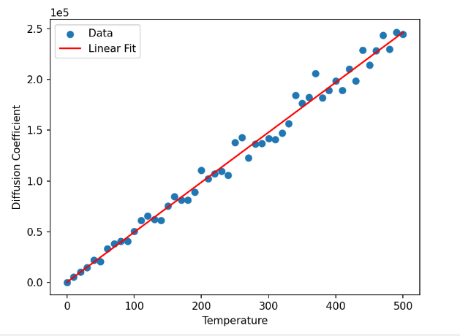
Slope: The slope is 493.10, indicating the effect of a one-unit change in temperature on the diffusion coefficient. The relatively large absolute value of the slope suggests a significant influence of temperature on the diffusion coefficient.

Intercept: The intercept is 77.47, representing the diffusion coefficient at a temperature of zero. However, in practical terms, this may not have a meaningful interpretation since temperatures are not typically zero.

R-squared: The R-squared value is 0.988, very close to 1. This indicates a strong linear relationship between temperature and the diffusion coefficient, with approximately 98.8% of the variability in the diffusion coefficient explained by the linear regression model.

P-value: The P-value is very close to zero (9.72e-49), indicating a high level of significance for the slope. This means we can reject the null hypothesis that the slope is zero, implying a significant impact of temperature on the diffusion coefficient [20].

3 Conclusion

This research uses Brownian motion simulation to calculate the relationship between temperature and diffusion coefficient in limited computing resources. With the 1-D random walk model, it makes recommendations for simulation timing, direction and particle numbers. The conclusion comes that the diffusion coefficient increases as the temperature increases, which follows a linear relationship. This research provides examples of using Brownian model to simulate multi particles system. It provides a solution for particle simulation with large volume or limited computing resources.

However, it is important to acknowledge certain limitations in the current study. The Brownian motion algorithm, while effective, may still benefit from streamlining to enhance computational efficiency. Additionally, future research endeavors could focus on achieving more precise simulations while maintaining the same level of computational complexity. This would contribute to a more nuanced understanding of molecular dynamics, particularly in scenarios involving intricate interactions and diverse environmental conditions. These aspirations pave the way for continued advancements in the field, offering opportunities for refinement and innovation in Brownian motion simulations.

References

[1]. Frenkel, D., & Smit, B. (2023). Understanding molecular simulation: from algorithms to applications. Elsevier.
[2]. Hartley, G. S., & Crank, J. F. (1949). Some fundamental definitions and concepts in diffusion processes. Transactions of the Faraday Society, 45, 801-818.
[3]. Maxwell, J. C. (1867). IV. On the dynamical theory of gases. Philosophical transactions of the Royal Society of London, (157), 49-88.
[4]. Einstein, A. (1905). On the motion of small particles suspended in liquids at rest required by the molecular-kinetic theory of heat. Annalen der physik, 17(549-560), 208.
[5]. Schilling, R. L., & Partzsch, L. (2014). Brownian motion: an introduction to stochastic processes. Walter de Gruyter GmbH & Co KG.
[6]. Ratcliff, L. E., Mohr, S., Huhs, G., Deutsch, T., Masella, M., & Genovese, L. (2017). Challenges in large scale quantum mechanical calculations. Wiley Interdisciplinary Reviews: Computational Molecular Science, 7(1), e1290.
[7]. Mazo, R. M. (2008). Brownian motion: fluctuations, dynamics, and applications (Vol. 112). OUP Oxford.
[8]. Codling, E. A., Plank, M. J., & Benhamou, S. (2008). Random walk models in biology. Journal of the Royal society interface, 5(25), 813-834.
[9]. Einstein, A. (1956). Investigations on the Theory of the Brownian Movement. Courier Corporation.
[10]. Karlin, S. (2014). A first course in stochastic processes. Academic press.
[11]. Codling, E. A., Plank, M. J., & Benhamou, S. (2008). Random walk models in biology. Journal of the Royal society interface, 5(25), 813-834.
[12]. Witte, R. S., & Witte, J. S. (2017). Statistics. John Wiley & Sons.
[13]. Yap, B. W., & Sim, C. H. (2011). Comparisons of various types of normality tests. Journal of Statistical Computation and Simulation, 81(12), 2141-2155.
[14]. Augustin, N. H., Sauleau, E. A., & Wood, S. N. (2012). On quantile quantile plots for generalized linear models. Computational Statistics & Data Analysis, 56(8), 2404-2409.
[15]. Uhlenbeck, G. E., & Ornstein, L. S. (1930). On the theory of the Brownian motion. Physical review, 36(5), 823.
[16]. Sekimoto, K. (1998). Langevin equation and thermodynamics. Progress of Theoretical Physics Supplement, 130, 17-27.
[17]. Zuckerman, D. M. (2010). Statistical physics of biomolecules: an introduction. CRC press.
[18]. Dieker, T. (2004). Simulation of fractional Brownian motion (Doctoral dissertation, Masters Thesis, Department of Mathematical Sciences, University of Twente, The Netherlands).
[19]. Montgomery, D. C., Peck, E. A., & Vining, G. G. (2021). Introduction to linear regression analysis. John Wiley & Sons.
[20]. Seber, G. A., & Lee, A. J. (2003). Linear regression analysis (Vol. 330). John Wiley & Sons.
Cite this article
Wu,X. (2024). Using Brownian model to study the effect of temperature on diffusion coefficient. Theoretical and Natural Science,36,48-57.
Data availability
The datasets used and/or analyzed during the current study will be available from the authors upon reasonable request.
Disclaimer/Publisher's Note
The statements, opinions and data contained in all publications are solely those of the individual author(s) and contributor(s) and not of EWA Publishing and/or the editor(s). EWA Publishing and/or the editor(s) disclaim responsibility for any injury to people or property resulting from any ideas, methods, instructions or products referred to in the content.
About volume
Volume title: Proceedings of the 2nd International Conference on Mathematical Physics and Computational Simulation
© 2024 by the author(s). Licensee EWA Publishing, Oxford, UK. This article is an open access article distributed under the terms and
conditions of the Creative Commons Attribution (CC BY) license. Authors who
publish this series agree to the following terms:
1. Authors retain copyright and grant the series right of first publication with the work simultaneously licensed under a Creative Commons
Attribution License that allows others to share the work with an acknowledgment of the work's authorship and initial publication in this
series.
2. Authors are able to enter into separate, additional contractual arrangements for the non-exclusive distribution of the series's published
version of the work (e.g., post it to an institutional repository or publish it in a book), with an acknowledgment of its initial
publication in this series.
3. Authors are permitted and encouraged to post their work online (e.g., in institutional repositories or on their website) prior to and
during the submission process, as it can lead to productive exchanges, as well as earlier and greater citation of published work (See
Open access policy for details).