


1. Introduction
1.1. Quark-Gluon Plasma
Believed to be the most fundamental states of matter, the Quark-Gluon Plasma (QGP) consists only of individual quarks and gluons. Current theory suggests that QGP is the state of matter that exists immediately after the Big Bang and can be replicated under certain conditions in particle colliders, in which extreme temperatures and pressures are reached. Under such conditions the quarks and gluons, normally confined within hadrons, are released by the weakening of the strong force. The properties of QGP are similar to a perfect fluid, exhibiting low viscosity and strong collective behavior. As these conditions are most often reproduced in heavy ion collisions, instrumental studies of QGP are conducted largely at the Relativistic Heavy Ion Collider (RHIC), and the Large Hadron Collider (LHC) at CERN. Also widely believed to be the state of matter that existed shortly after the Big Bang, the study of QGP can give insight into the strong force, the fundamental state of matter, and the early state of the cosmos. Particle colliders and detectors use simulation and instrumental experiments as ways of studying the various properties of QGP. In this article, we examine a set of simulated data with Au-Au heavy ion collisions and the detected results.
1.2. Particle Detectors
As particle detectors cannot directly detect the position of particles, determination of the positions of energy fluctuations on multiple layers of cylindrical detectors is an alternate way. From this data of positions, the detector calculates the path of particles. For the reconstruction of events, the detector adopts a variant of spherical coordinates instead of Cartesian coordinates, with the polar axis (also the “beam axis”) perpendicular to the collision plane [1, 2], and the origin set at the geometric center of the cylindrical detectors. Through the collected data and a transformation function to be calculated in section 2.1, the events are reconstructed.
1.3. Pseudorapidity
The distribution of \( θ \) with respect to the beam axis is not uniform, which means that generating histogram of \( θ \) would not yield a flat distribution, resulting in difficulties for further analysis. Thus, the transformation for pseudorapidity ( \( η \) ) is introduced:
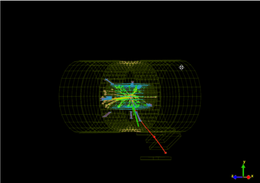
Figure 1. z-axis view of particle collider.
\( η= -ln(tan{(\frac{θ}{2})}) \)
Of which the reverse formula, used when the given values of the simulated ROOT data are in pseudorapidity form:
\( θ= 2 \cdot arctan{(exp{(-η)})} \)
And the preliminary conversion formulas are complete. Note that for this particular simulated experiment, \( η \) ranges from \( -1 \) to \( 1 \) , limited by the dimensions of the detectors.
1.4. The Centrality \( {v_{0}} \)
During collisions, the ions exhibit different modes [3-6]. One of the parameters separating the modes is the impact parameter \( {v_{0}} \) , describing the centrality. Its value is measured as the distance between the center of the two colliding nuclei [2], which implies that a smaller value of \( {v_{0}} \) means a more head-on collision, while a larger value would mean that the collision is more peripheral. The number of particle hits can be drastically different depending on the value of \( {v_{0}} \) , thus separation of data in the order of \( {v_{0}} \) is needed.
2. Method for Research
2.1. Mathematical Model
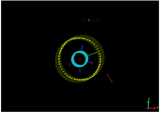
Figure 2. \( x \) -axis view of particle collider.
To construct a clear model of the collider, we first need to construct a coordinate system. Defining A as a detected point of energy fluctuation, a hypothetical cube with OA as the body diagonal is constructed, and edges parallel or perpendicular to the z-axis. Thus, the Cartesian coordinate \( (x,y,z) \) can be geometrically interpreted, as shown in fig. 2, determining the position mentioned above. And with further calculations in trigonometry, we can produce the transformation vector function as follows:
\( [\begin{matrix}x \\ y \\ z \\ \end{matrix}]=R\cdot [\begin{matrix}sin{(φ)} \\ \sqrt[]{{cos^{2}}{(φ)\cdot {sec^{2}}{(θ)-1}}} \\ cos{(φ)} \\ \end{matrix}] \) .
In which \( φ \) and \( θ \) are defined in the introductory material. Through a reverse function with trigonometry, the ROOT data in \( (R,η, φ) \) mode can also be converted:
\( [\begin{matrix}R \\ θ \\ φ \\ \end{matrix}]=[\begin{matrix}R \\ arctan {(\frac{\sqrt[]{{x^{2}}+{y^{2}}}}{z})} \\ arctan{(\frac{x}{y})} \\ \end{matrix}] \)
Which leads to the completion of the mathematical model for the particle detector. Note that R is a determined constant, thus there is no need for conversion.
2.2. Vertex Determination
To determine the vertices of events, we would need to calculate the differences between the \( φ \) and \( η \) values first.
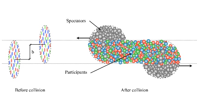
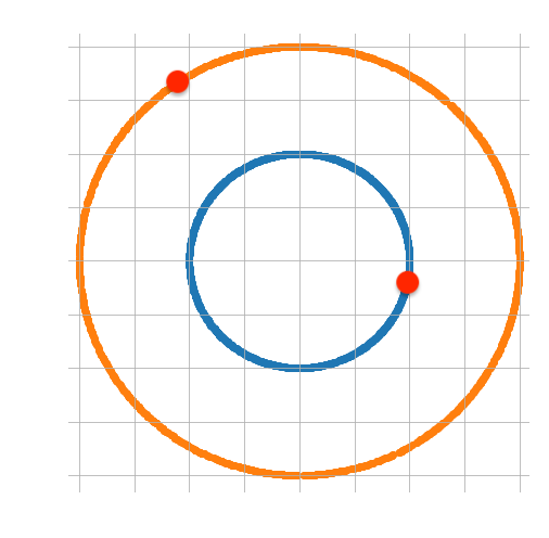
Figure 3. Geometric interpretations of \( {v_{0}} \)
2.3. Vertex With Centrality
In order to investigate multiplicity for different types of Au+Au collisions, we inspected the centrality parameter \( {v_{0}} \) of all events, ranging from peripheral collision of \( {v_{0}} \) =406 to central collision with \( {v_{0}} \) =10384.
To give an overview, we plotted a histogram of \( {v_{0}} \) values for all events, provided that we log scaled the frequency to obtain the impact parameter (see figure 4). The histogram meets our expectation such that there are a lot more events with smaller \( {v_{0}} \) values comparing to those with bigger \( {v_{0}} \) values. We then classified all collision events into 11 categories according to collision centrality, namely 0-5%, 5-10%, 10-20%, 20-30%, 30-40%, 40-50%, 60-70%, 70-80%, 80-90% and 90-100%.
In order to study Au+Au collisions in further detail, we chose to analyze the multiplicity of 10 events in each category of collision centrality. Multiplicity helps determine properties of the Au+Au collisions and is related to collision energy and number of participants in collisions. (In this case, the number of nucleons that are involved in the collision.) As shown in figure 3, one should note that the more central a collision is (high \( {v_{0}} \) value), the larger number of participants would be created, thus less spectators, which are nucleons that aren’t involved and would just keep following the path of the beam.
Prior to expanding on the analysis of multiplicity, please note that this specific set of data was generated from three layers of
detectors, layer 0, 1 and 2; therefore, when analyzing the data, we used (delta eta) and (delta phi) values between layer 0 and 1, 0 and 2, 1 and 2 respectively to get three sets of results, which were then averaged out to show an overall trend.
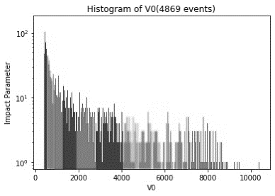
Figure 4. Histogram of \( {v_{0}} \)
The sideband method is introduced to study multiplicity. Procedures of the sideband method consists of choosing sideband and signal regions for \( Δφ \) according to a certain range of \( Δη \) on our \( Δφ \) - \( Δη \) scatter diagram shown in figures 10-13. We defined the signal region as events that fall into the range -0.1 \( ≤ Δη≤ \) 0.1, and sideband region as those satisfy -0.2 \( ≤ Δη \lt \) -0.1 or 0.1 \( \lt Δη ≤ \) 0.2, for which the sideband regions contain background signal particles, and the signal regions have signal and background particles. We subtracted the sideband region form the signal region to give an estimate of counts of participants. As shown in figures 10, 11, 13 and 14, we plotted histograms for \( Δφ \) in sideband region, signal region and of which after subtraction respectively for all 11 categories with 10 random sets of data. The triangular base represents background counts, whereas the peak at \( Δφ =0 \) above the triangular base is considered to only contain the signal particles. Counts at \( Δφ =0 \) inside the triangle was eliminated, the reason being there are other Standard Model processes going on in the background that are similar to those that produced the signal data we desire. The total count is obtained by adding up counts within the signal region of -0.1 \( ≤ Δφ ≤ \) 0.1.
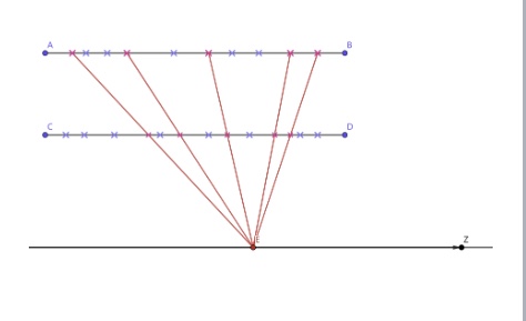
Figure 5. A sample of the idea of Hough transform
Figures 12 and 15 illustrate histograms of the sideband region, signal region and the peak of a different category in terms of centrality. As shown, a lower \( {v_{0}} \) value results in a lower count and a flatter sideband region. We believe that since the collisions are getting more peripheral, not only the number of participants decreases, but also the proportion of background counts distributed around \( Δφ =0 \) that confuse with the signal counts.
However, the sideband method only gives a rough estimation; to lower the uncertainty, we normalized the result to produce a much more precise estimation of multiplicity. For normalization, we introduced \( α \) , which is a constant that represents the ratio of background counts in signal region to that in sideband region. It is calculated via:
\( α=\frac{sum of counts in signal region}{sum of counts in sideband region} \) ,
|
|
Figure 6. A sample of the idea of Hough transform | Figure 7. Histogram with \( z=11 \) |
with \( -2π≤Δφ \lt -1 \) or \( 1≤Δφ≤2π \) )). We then multiplied each individual count of (delta phi) from the sideband region by alpha to mimic the background count of which in the signal region. The subtraction of normalized sideband region from the original signal region is then carried out and a peak with less noise is produced as shown in figure15. The trend of signal counts with descending \( {v_{0}} \) remains the same.
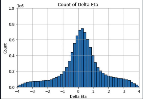
In a particle collier, the two original particles that are about to hit lay on the same position of a cross section plane off the collider from the side, which means that the x and y axis of these two particles are irrelevant. Therefore, only the z axis needs to be analyzed in order to find the position of the collision point. The data set contains the positions of the hits on the layers of the collider by the released particles from the collision. This relative position of the hits is based on the midpoint of the collider. Since there are 3 layers on the collider that detects these hits, we choose to separate the 3 layers into 3 sets of 2 and analyze the deltas separately. We tried to find all the combinations of the hits on the 2 layers, draw the line that pass through the 2 hits representing a possible particle that create these two hits, and find the point where an extreme large number of lines suddenly come to an interaction and that point should be the place where the collision took place. However, this strategy is too complicated with the amount of data we got from a collision, so we came up with another strategy based on the idea of Hough transform making the process more efficient and the result more reliable. In the strategy, a hypothesis point of collision called u is set on the z axis. If use E as a reference point for the position of the hits, the z axis of the hits changes to be relative to E and convert this new set of data into a simpler form to analyze—eta and phi. We can then get all the combinations of delta eta and delta phi and since both eta and phi are angle values for the line that connects the hit and the origin, which is E in this case, the smaller the absolute value of delta eta and the absolute value of delta phi is the closer the line crossing the 2 hits is to u. Next, take out the delta etas and draw a histogram based on its values to make the results clearer. However, the look of the graphs turns out to be different from what was expected, so we encountered delta phi in the process. After getting all delta eta and delta phi, add in a process that removes all the combination of two hits with a delta phi outside the range of [-0.1, 0.1] since the 2 hits for these \( Δφ \) are not created by the same particle. We can then repeat the rest of the process again and find the E with an extreme peak in the histogram and that should be the correct collision point. On the basis, the other 2 combinations of layers can be used to verify the E we got from 1 combination of layers.
|
|
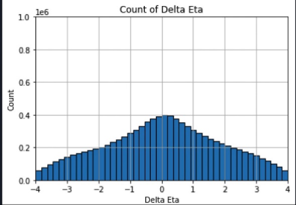
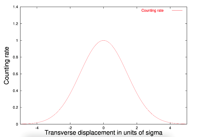
Figure 8. Histogram with \( z=-2 \) | Figure 9. Theoretical Distribution of \( Δφ \) |
3. Conclusion
During the process of our research, we constructed a satisfactory quantitative model of a particle detector, and through the Hough transform and classification process with \( {v_{0}} \) , determined that the vertex of events is relatively close to the geometric center of the detector. In the future, we wish to examine the events in groups corresponding to the \( {v_{0}} \) values, determining the correlation between the centrality value and the vertex position. Also, optimization of the algorithm calculating the vertex is needed, which would improve the accuracy of the measurements, helping more thorough investigations into the properties of QGP.
Acknowledgements
Jiarui Liu, Zisheng Yan, and Rongquan Zhou contributed equally to this work and should be considered co-first authors. Special thanks to Professor Gunther Roland from the MIT Physics Department for dedicated and detailed guidance on the team’s research.
References
[1]. Jacak, B, and Steinberg, P. Creating the Perfect Liquid in Heavy-Ion Collisions. United States: N. p., 2010. Web. doi:10.1063/1.3431330.
[2]. CMS Collaboration, “Multiplicity and transverse-momentum dependence of two- and four-particle correlations in pPb and PbPb collisions.” Phys. Lett. B 724 (2013) 213. Web.
[3]. Alver and Roland, “Collision Geometry Fluctuations and Triangular Flow in Heavy-Ion Collisions.”Phys.Rev.C81:054905,2010. Web. DOI: 10.1103/81.054905.
[4]. Heinz, “Concepts of Heavy-Ion Physics.” CERN Yellow Report CERN-2004-001, pp.127-178.DOI: 10.48550/ 0407360.
[5]. d’Enterria, “Quark-Gluon Matter.” DOI: 10.1088/0954-3899.
[6]. Centrality determination in heavy-ion collisions with the LHC detector [OL]. Aaij, Roel et al.
Cite this article
Liu,J.;Yan,Z.;Zhou,R. (2024). A study of collision vertex and centrality of simulated Au-Au Ion collision data sets at 200GeV . Theoretical and Natural Science,34,330-336.
Data availability
The datasets used and/or analyzed during the current study will be available from the authors upon reasonable request.
Disclaimer/Publisher's Note
The statements, opinions and data contained in all publications are solely those of the individual author(s) and contributor(s) and not of EWA Publishing and/or the editor(s). EWA Publishing and/or the editor(s) disclaim responsibility for any injury to people or property resulting from any ideas, methods, instructions or products referred to in the content.
About volume
Volume title: Proceedings of the 3rd International Conference on Computing Innovation and Applied Physics
© 2024 by the author(s). Licensee EWA Publishing, Oxford, UK. This article is an open access article distributed under the terms and
conditions of the Creative Commons Attribution (CC BY) license. Authors who
publish this series agree to the following terms:
1. Authors retain copyright and grant the series right of first publication with the work simultaneously licensed under a Creative Commons
Attribution License that allows others to share the work with an acknowledgment of the work's authorship and initial publication in this
series.
2. Authors are able to enter into separate, additional contractual arrangements for the non-exclusive distribution of the series's published
version of the work (e.g., post it to an institutional repository or publish it in a book), with an acknowledgment of its initial
publication in this series.
3. Authors are permitted and encouraged to post their work online (e.g., in institutional repositories or on their website) prior to and
during the submission process, as it can lead to productive exchanges, as well as earlier and greater citation of published work (See
Open access policy for details).
References
[1]. Jacak, B, and Steinberg, P. Creating the Perfect Liquid in Heavy-Ion Collisions. United States: N. p., 2010. Web. doi:10.1063/1.3431330.
[2]. CMS Collaboration, “Multiplicity and transverse-momentum dependence of two- and four-particle correlations in pPb and PbPb collisions.” Phys. Lett. B 724 (2013) 213. Web.
[3]. Alver and Roland, “Collision Geometry Fluctuations and Triangular Flow in Heavy-Ion Collisions.”Phys.Rev.C81:054905,2010. Web. DOI: 10.1103/81.054905.
[4]. Heinz, “Concepts of Heavy-Ion Physics.” CERN Yellow Report CERN-2004-001, pp.127-178.DOI: 10.48550/ 0407360.
[5]. d’Enterria, “Quark-Gluon Matter.” DOI: 10.1088/0954-3899.
[6]. Centrality determination in heavy-ion collisions with the LHC detector [OL]. Aaij, Roel et al.