1. Introduction

Determining how large ions behave when collide under relativistic conditions is key to the understanding of the subatomic world. This study aimed to find the average number of particles produced from gold ion collisions [1] at √S_NN = 200 GeV by working with data from the ALICE experiment with azimuthal angle acceptance ±π and pseudorapidity interval |η| < 1 [2], and then compare how this multiplicity varies with the centrality of collisions. By understanding how the collision results vary with the position of the colliding ions, we can hopefully gain a better picture of the transient nature of the quark-gluon plasma produced when partons in a nucleus become deconfined. The collider will first be introduced together with the study of the interested variables. Then, the sideband method employed to determine charged particle multiplicity will be presented with methods of normalization, and finally combined with the analysis of centrality.

2. The ALICE detector

The ALICE (A Large Ion Collider Experiment) detector is dedicated to studying matter under the influence of the strong force at the LHC (Large Hadron Collider). The experiment focused especially on understanding the production of the quark-gluon plasma, the fifth state of matter in the form of a dense and hot mixture of deconfined quarks and gluons. Energy is interchangeable with mass, meaning matter can be created from energy and vice versa. The beam accelerated close to the speed of light inside the detector will be able to create matter when it strikes. Fig.1 shows the computer-generated “cut-away” view of the ALICE detector.

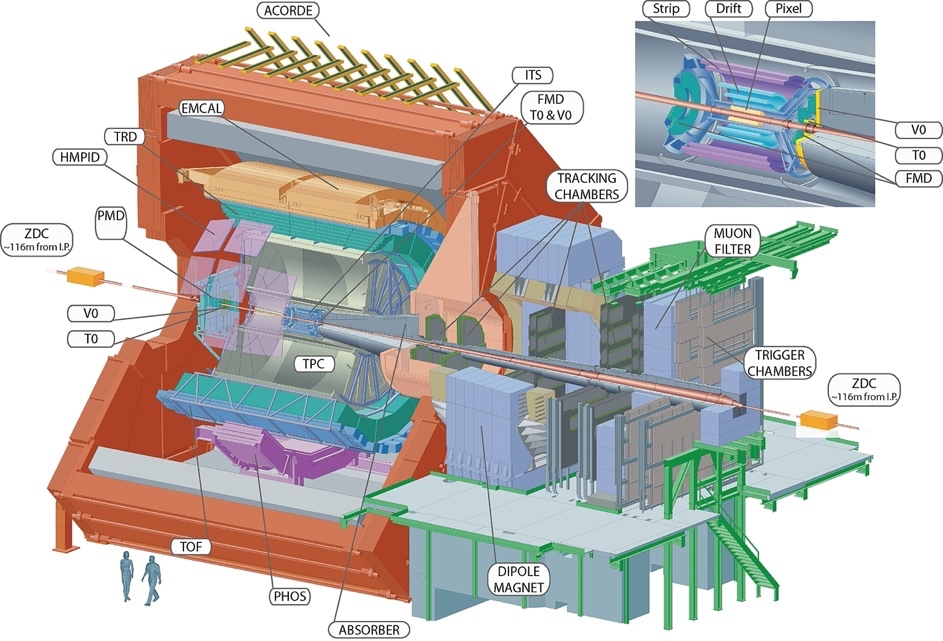
Figure 1. Schematics of the ALICE subdetectors [3].

The ALICE Detector has 18 sub-detectors. The central collision track is first surrounded by the tracking system, then a layer of electromagnetic and hadronic calorimeters which determines the types of interactions taking place by looking at the energy deposited by different types of particles. At the outermost layer, there is the muon spectrometer, where the decay of the heavy quarkonium to produce muons and antimuons is studied [4]. To determine the charged particle multiplicity, the Inner Tracking System (ITS) and the Time Projection Chamber (TPC) become particularly useful (See Fig.1). The ITS consists of three layers of silicon detectors: The Silicon Pixel Detector (SPD), the Silicon Drift Detector (SDD), and the Silicon Strip Detector (SSD). Each of these three layers contains two sub-layers and are all responsible for suggesting the position of the particles being produced. The TPC is sensitive to all charged particles, as they ionise the gases in the chamber and let out the electrons, which helps to identify those that carry an electrical charge from electrically neutral products [5].

3. Relevant Variables

The following measurements inside the ALICE detector are studied to determine the charged particle multiplicity (See Fig.2):

• ɸ: azimuthal angle. The angle of the particle trajectory in the plane transverse to the beam direction.

• θ: polar angle between the direction of the momentum of the particle with the positive beam axis.

• η: pseudorapidity, it is related to θ by the equation \( η=-ln⁡(tan{\frac{θ}{2}}) \) [6].

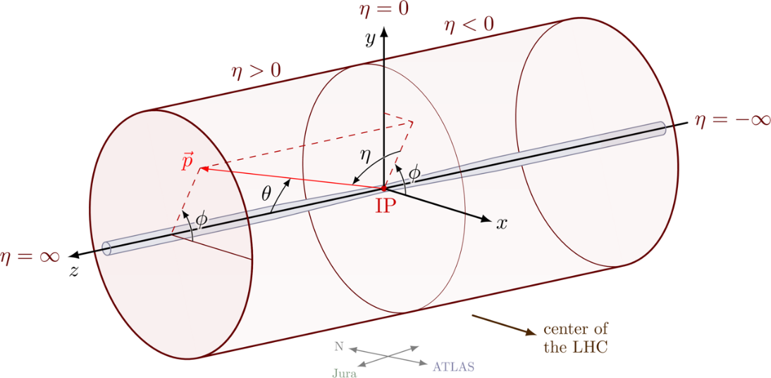
Figure 2. CMS coordinate system describing a cylindrical detector [7].

The subsequent section details a methodical approach to converting data into useful forms. The methodology employed in this analysis involves a systematic process of data separation and conversion to facilitate a comprehensive understanding of particle multiplicity. The given raw data, captured within a ROOT file format, serves as the canvas from which specified data is evaluated, and is converted into a more accessible text file for further analysis.

The first phase of our methodology centres on the separation of the converted data. The converted text file contains 5000 recorded events encompassing both background noise and genuine particle hits. To discern the interested hits and to organise them, two methods could be applied: splitting by reading “double integers” and the “jump split” method.

• Splitting events with double integers takes advantage of the fact that every event header in the file is a line consisting of two non-negative integers. Separation by double integer reads one line of the file at a time and splits it into distinct events each time it detects a pair of double integers in a line.

• Jump split on the other hand can be applied to more general forms of data. In the converted file, the headers of the events have four columns; the first column is the event number, the second column is the signal number, the third column is a float parameter (this means the first method may not work effectively), and the fourth column is the impact parameter. By utilizing the jump split method, it reads the number of signals recorded from the second column, n. This gives knowledge to the next n lines being the signal of this specific event, and this can be repeated with all other events to extract individual events. Having isolated the events, the data is further segmented into individual layers – the 3 silicon layers in the ITS of the ALICE detector (later represented as layer 0,1,2 respectively from inner to outer). The layer-based segmentation disentangles the raw data, which not only facilitates a more structured representation of particle trajectories but also enables the identification of particle interactions at varying depths within the detector. The separation of these layers is crucial to regrouping later in the study. The next step involves the removal of redundant integer columns. Since we have separated the individual layers, integer identification is no longer required. By eliminating this superfluous integer column, we enhance the interpretability and usability of the data for visualization and analysis. The final step entails the separation of variables. As we have converted out x, y, and z coordinates to angles φ and η, we now utilised the comma to differentiate the two. By splitting, we stake out the individual data points and can verify the validity of the data – later done by examining the distributions of φ and η.

Having separated and structured our data, we turn our focus to the analysis of phi (φ) and eta (η) distributions. They are crucial in determining the positions and distribution of particles inside the detector. An analysis of the φ and η distributions involves binning the data into angular intervals and constructing a histogram that depicts the frequency of hits at azimuthal angle range (-π, π) and pseudorapidity range (-1,1). Intriguingly, both histogram distributions exhibit a nearly flat distribution, as shown in Fig.3 and Fig.4. This uniformity comes from a principal attribute of the detector itself – an equal probability of receiving hits from our range for azimuthal angles and pseudorapidity. As the collision transpires, an ensuing cascade of particles permeates the detector, resulting in an equal likelihood of particle interactions occurring from all interested directions. This property of the detector engenders flatness in the distributions, capturing the essence of the initial impact’s omnidirectional consequences.

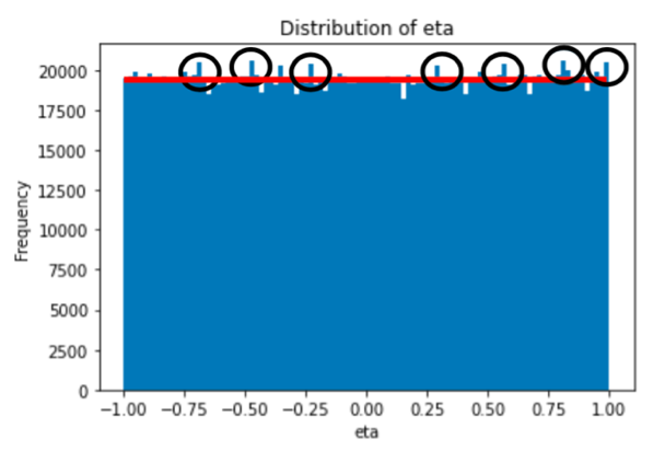
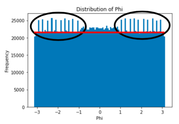
However, within this overarching uniformity, we encounter an abundance of nuances. Delving deeper, we unveil small, localised deviations disrupting the otherwise uniform distribution. These deviations, although seemingly disruptive, are marks of background noise – an assortment of insignificant signals that intrude upon the data due to experimental imperfections, extraneous sources, and the sensitive nature of the detector renders it susceptible to registering false alarms. These inconspicuous spikes necessitate diligent scrutiny and careful filtering, ensuring that the genuine insights encapsulated within the distribution remain untainted by these minor perturbations – later resolved by methods of normalisation.

4. Trajectory tracking

After obtaining the value of pseudorapidity and azimuthal angle for each recorded hit on each layer, we need to construct the paths of the particles by connecting the hits. The particles produced from high-energy collisions contain high kinetic energy and undergo little deviation in path direction when penetrating the three layers of the ITS. Spatially, the three hits belong to the same particle and can be connected to form a nearly straight line, and we will call it a “path” in this study. Finding the number of these paths has the same physical significance as finding the number of particles produced. The three hits forming the path will give close values of η (±0.1) and φ (±0.1π) as any part of a straight line forming the same angle with the same reference axis. Therefore, we can introduce a change of spatial position of hits between layers, Δη and Δɸ, such that:

\( ∆η=η1-η2 \)

\( Δϕ=ϕ1-ϕ2 \)

The reason why we accept small differences between pseudorapidity and azimuth comes from the consideration that magnetic fields [8] in the detector can give rise to mild variations in path directions when a particle travels.

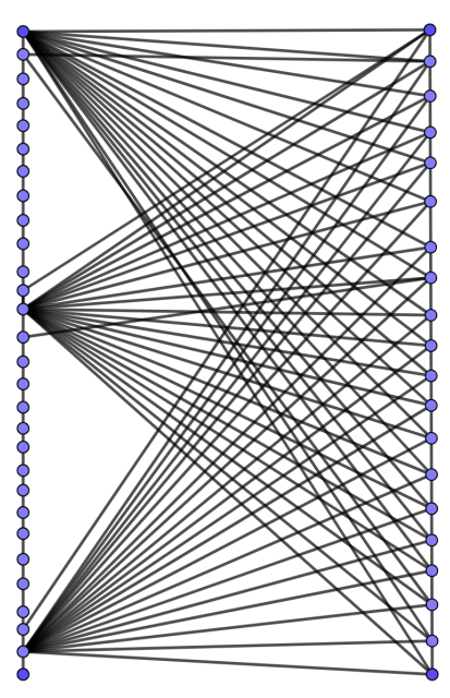
Figure 5. Visualising the calculation of Δη and Δɸ for some hits between two layers (rows).

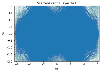
Since there is no obvious and direct sequential correspondence between the two layers of data recorded by the detector, we need to subtract the eta and phi values of each point on one layer from the η and ɸ values of each point on the other layer respectively (shown in Fig.5) to ensure that the correct “beam” left by the same charged particle is found. Take event 1 of the data for example, the visualization of Δη and Δɸ between layer2&1 calculated using η and ɸ values on layer1 and layer2 are shown in Fig.5 and Fig.6.

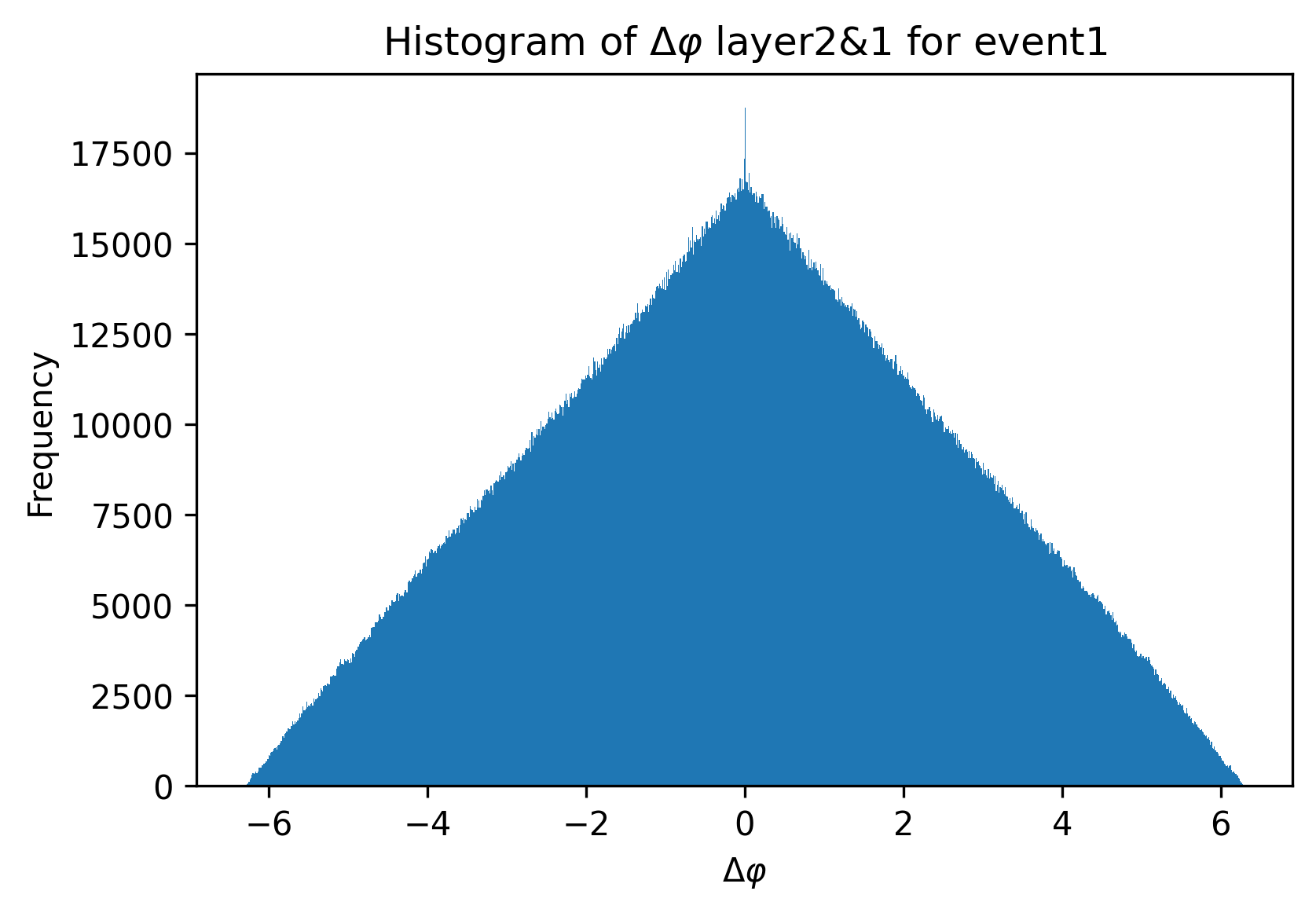
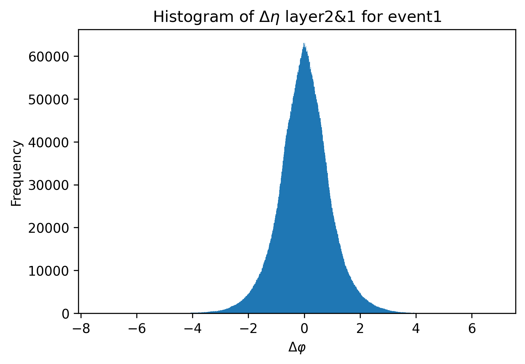
From the figures above, we can see that at around Δη and Δɸ equal 0, a certain range of bins forms a sharp spike, indicating the number of signals on layer2 and layer1 that successfully form a beam on the corresponding spatial vector (η or ɸ). By later analysis like considering Δη and Δɸ together, it is reasonable to get the estimated number of particles produced in the collisions.

However, it is key to discuss the limitation of this Δ calculation. The first is that since the detector often detects background noises that cannot be effectively eliminated, the noises are also treated as data points. Consequently, these noises can also be involved in our delta calculations due to the permutation form. In some special cases, when a noise from one layer happens to form a beam with a data point from another layer (Δ is within a very small range of 0), then we risk incorrectly counting that a charged particle, which leads to a certain degree of overestimation of charged particle multiplicity. Furthermore, due to the limitations of the algorithm and the large computational amount of permutation, it is not possible to consider Δ of three layers at the same time. Therefore, our main solution in the later stage is to combine any two of the three layers until the average value is obtained after the final Δ and multiplicity calculation. We believe that this estimation method can be effective because there is only one point of collision for the same event, so there should be no significant difference in spike heights between any two of the three layers. Finally, due to the natural property of Au+Au collision, we are dealing with a very large number of data points, and a visualization of these data points in a collider (vertically placed for convenience) tells the abundancy of data for even a single event (see Fig.8).

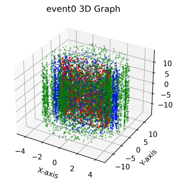
Figure 8. Visualisation of hits on the detector.

When the density is high, we suspect that there may be data points that are highly coincident or spaced less than 10^-4. These data points may be recorded by completely different products, but due to the permutation calculation, a delta that is very close to 0 will mainly lead to an inconspicuous spike since they are mainly distributed on both sides close to the bin representing 0, which may also lead to an overestimation of the number of particles produced since we consider a certain range of bins around 0 to be the effective bins.

5. The Sideband Method

5.1. Sideband definition

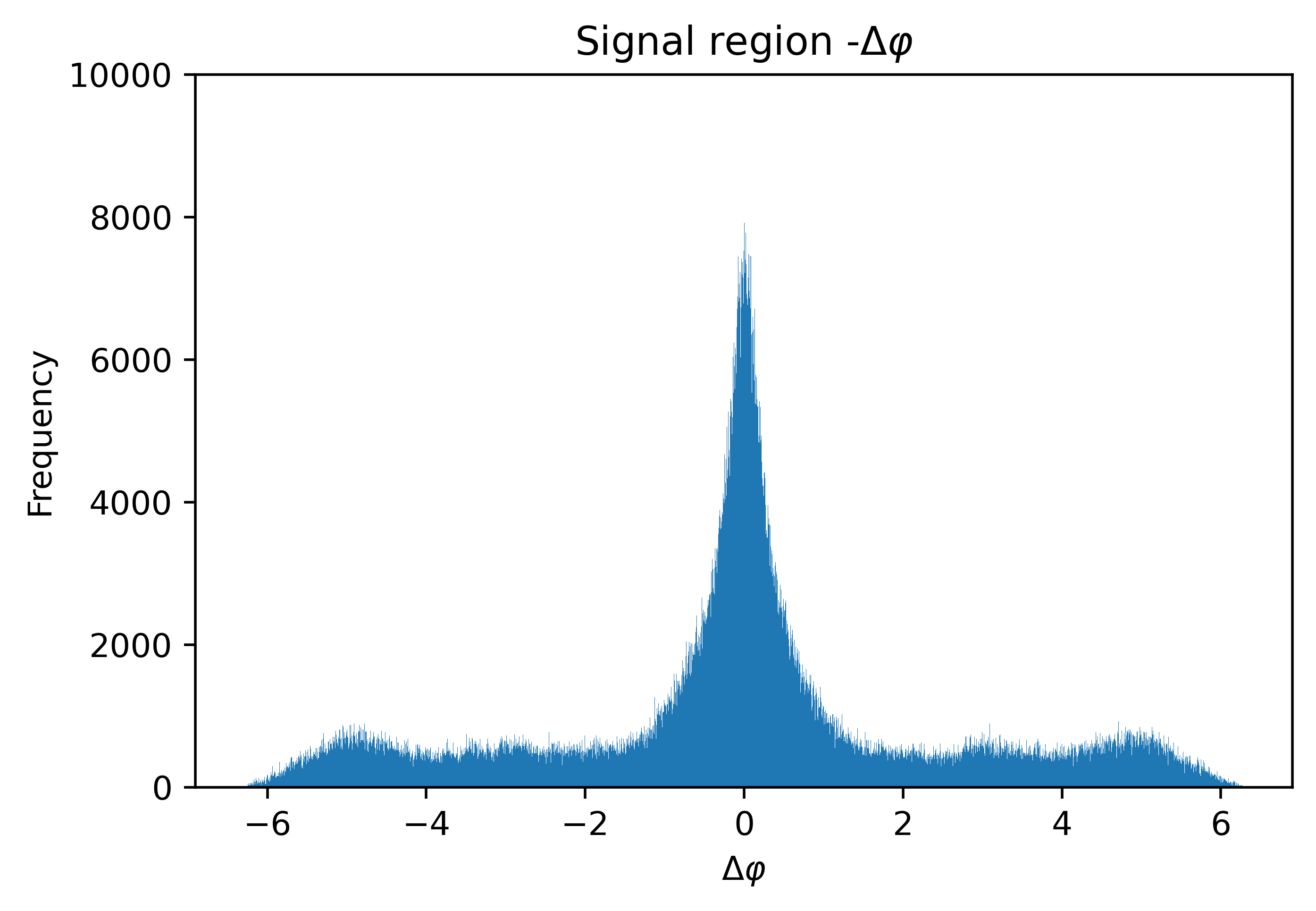
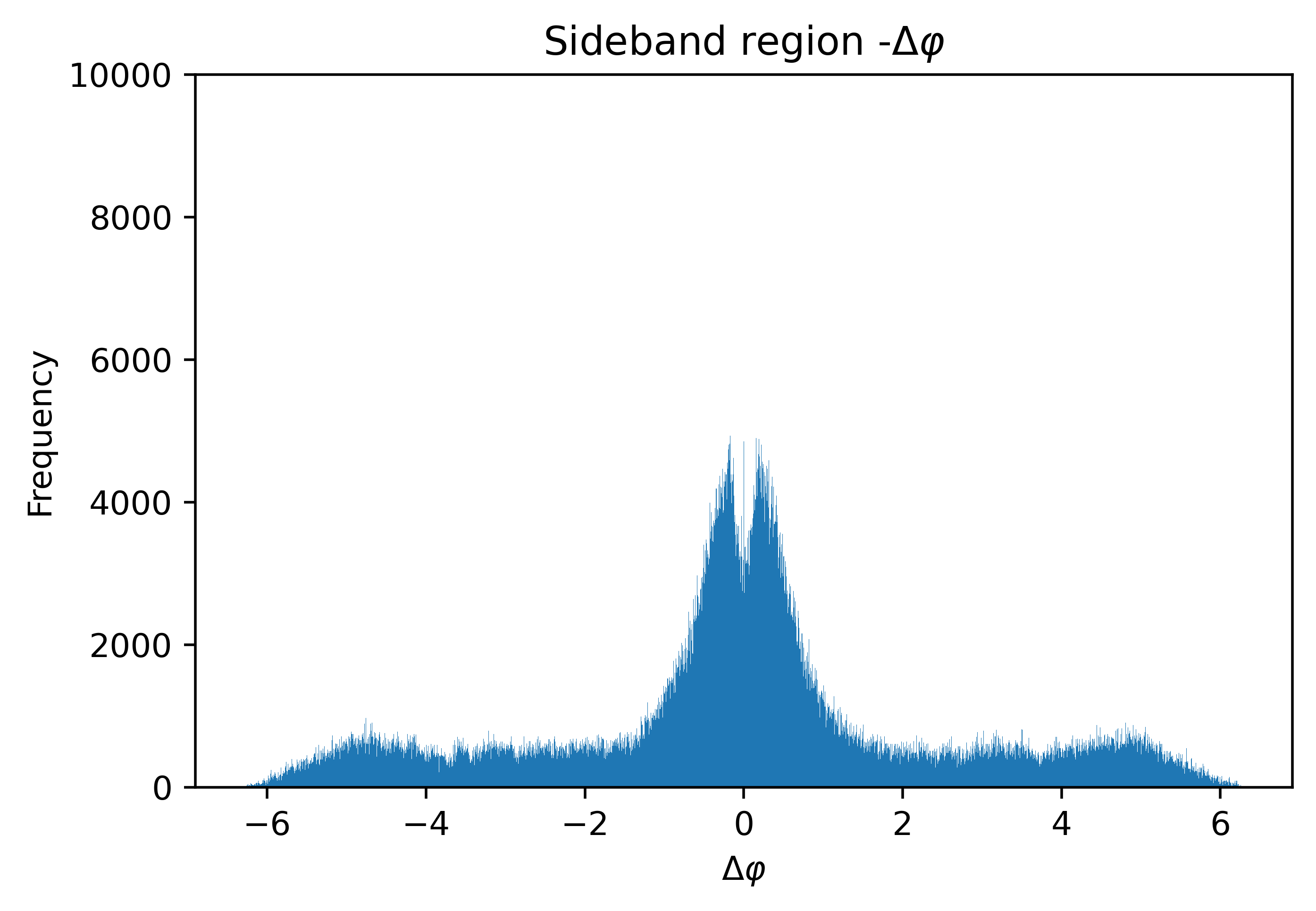
To find the average number of particles produced in a collision with rest mass energy = 200 GeV, it is imperative to find this number in each event first. The charged particle multiplicity is determined by steps of the sideband method, which involves the selection of regions around the known position of the signal and performing subtraction. In this study, we use this method with our Δη-Δɸ diagram and chose to extract data points of Δɸ within a range of Δη. This is done in such order because working with a limited pseudorapidity range of (-1,1) is easier compared to the azimuthal angle range of (-π, π). In this study, the detector collecting the data has three layers, named after 0, 1, and 2. There are three possible combinations of layers to give three different Δη and Δɸ for each event, from 2-0, 2-1, and 1-0. The differences become useful to confirm the multiplicity as we expect there to be a similar number of particles arriving at adjacent layers. Inside a detector, we understand that when Δη≈0 the particle is nearly perfectly ‘on-course’ after its production at the point of collision. After obtaining the plot of Δη-Δɸ, as shown in Fig.9, there is a noticeable concentration of data points at Δη≈0 and Δɸ≈0, which supports the assumption that most particles would be undeflected upon entering a new layer. The signal region can be defined by taking the (-0.10, 0.10) range, and the upper sideband region is in [0.10, 0.20) with the lower sideband in (-0.20, -0.10]. The two sideband regions are treated as one and thus two distributions can be plotted in the form of histograms, and Fig.10 and Fig.11 show the plot for the signal region and the sideband region for Δɸ respectively. The signal region contains both the interested signal and the background noise, as we select the region using only Δη≈0, which means Δɸ≈0 is not the only data point included in the distribution [9]. The sideband region contains just the background noises, and by choosing this suitable interval (the same number of bins as the signal region) we can perform a subtraction to find a close approximation of the signal:

\( {M_{signal}}≈{M_{signal region}}-{M_{sideband region}} \)

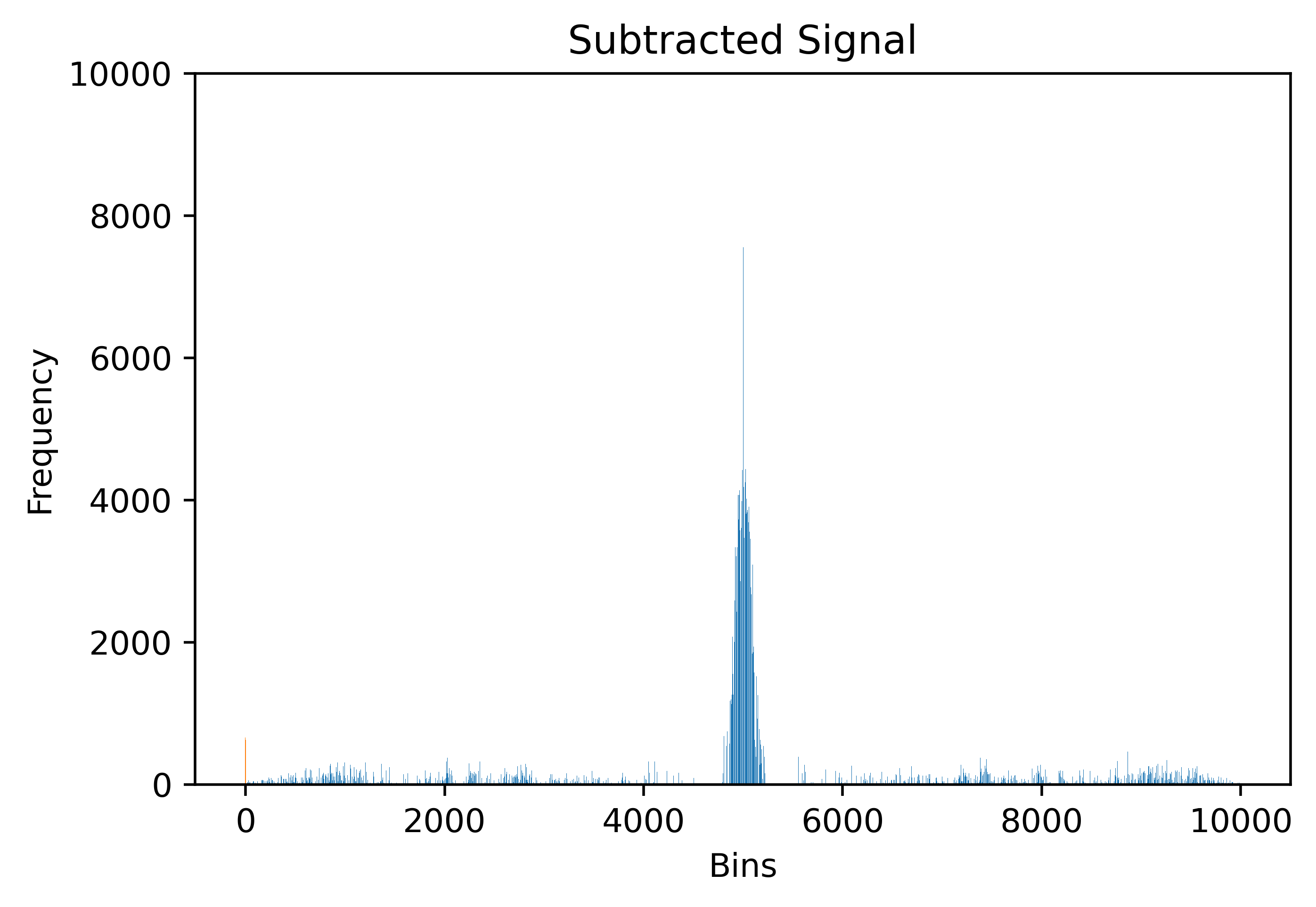
This gives only an approximation because we have assumed a uniform distribution of data points in the background, which means the backgrounds from the signal region and the sideband region can cancel each other out perfectly. In this study, the data from the ALICE experiment does not allow such an assumption, and mere subtraction would still leave the final signal spike mixed with mild background noises, as shown in Fig.12. Therefore, we introduce the normalization factor α.

5.2. Normalisation

The individual histogram heights of the sideband are subtracted from the signal band histogram. The subtraction process theoretically should produce a single spike. This happens because the data points of the selected sideband are underlying physical and background processes expected to be similar to those in the signal region; this expectation is proven by the similar triangular shape representing the background noise in both of the histograms. With only the graph of the peak, it is possible to determine a close estimation of the particles detected by the detector.

However, the shape of the signal band histogram (excluding the peak) could not be identical to that of the sideband. Discrepancies in data sets between the signal band and the sideband led to remaining background noises after subtraction. It is harder to determine the exact shape of the peak. In cases when the sideband has more data points of noise at zero, the peak will be smaller than the actual, and vice versa. Normalization processes were utilised to mitigate the quantity of background noise after the subtraction. Normalization involves the multiplication of the sideband data set with a certain multiplicity constant that molds the shape of the sideband data histogram to resemble the shape of the histogram of the signal band data. At the same time, the peak should not be influenced. The shape of the signal band histogram is not changed to preserve the value of the data points in the peak and minimise error formation. The multiplicity constant \( α \) is defined as,

\( α=\frac{\sum {y_{signal}}}{\sum {y_{sideband}}} \)

\( \sum {y_{sideband}} \) is the sum of the y value of sideband histogram bins of \( Δϕ \) or \( Δη \) value greater than 1 or less than -1, \( \sum {y_{signal}} \) is the sum of the y value of signal band histogram bins of \( Δϕ \) or \( Δη \) value greater than 1 or less than -1. The range chosen to include into the multiplicity constant is set to exclude the peak when calculating the multiplicity constant. Including the disproportionate height of the peak may cause an inaccurately larger multiplicity constant and higher y values of bins of normalised side band histogram. Subtraction will most likely cause the sum of the peak value to be smaller than the actual. Furthermore, the range of values of -1< \( Δη \) & \( Δϕ \) <1 is excluded during the calculation of \( α \) due to the intense fluctuation in the data.

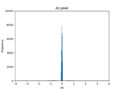
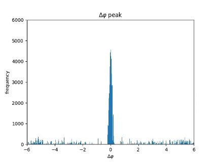
\( α \) was calculated as 0.995121 for \( Δϕ \) and 1.00767 for \( Δη \) . The side band histogram bin heights are all multiplied to \( α \) to produce the normalised histogram. By subtracting the y values of the normalised sideband dataset from those of the signal band data set, the peak for both \( Δϕ \) and \( Δη \) are obtained. Adding up the peak’s bin’s y values gives the value of the multiplicity of this specific event, being 869008.66 for \( Δϕ \) and 947679.98 for \( Δη \) .

6. Centrality

The important and final step of his study is to separate our 5000 events into different categories based on the centrality of collisions. In a collision between two ions, the degree of overlap between nuclei directly influences the number of participants recorded by the detector. In a particle accelerator, two plate detectors measure the energy, which scales directly with the number of primary particles generated in the collision and so therefore centrality. Centrality(v0) can be quantified using the impact parameter [10]. The larger the overlap the higher the average number of nucleons participating in the collision (N_part) [11].

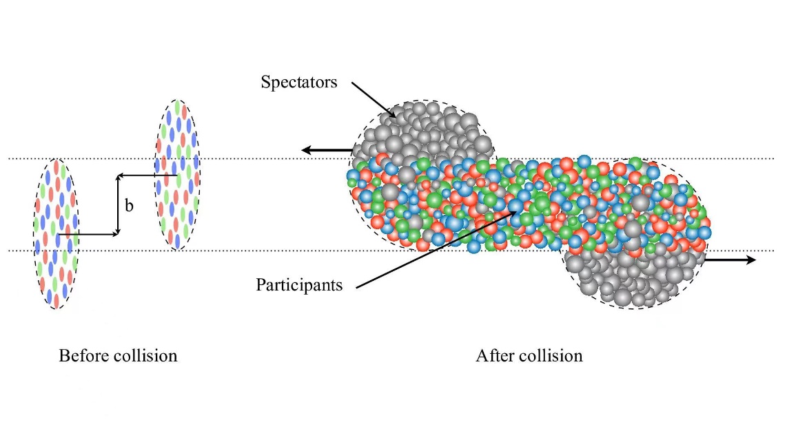
Figure 15. Presentation of the central and peripheral region of a collision between two ions.

Recall that when we just started to work on the new raw data which contains a complete recording of 4869 events and 131 events with only headers including the event number, the number of signals detected by the particle collider, a float parameter, and the impact parameter, we found out that the method we applied on both sets of previous data which contain no floats cannot be used anymore. The float parameter in each event makes it impossible to separate each event by judging the integer event header, therefore making further analysis impossible. By upgrading the algorithm and introducing the jump-split method, we can bypass the integer limitation of the headers. Jump-split is a method that should work which starts with reading the second parameter of the first line in the file (the number of signals detected by the particle collider) and jumps to that corresponding line. For instance, if the second parameter gives 3000, indicating that 3000 signals are detected and recorded and additionally the next 3000 lines should be “signal information”. This can give us the information that line 3001 is the beginning of the next event. We applied the jump-split method to our new data and found out that it failed to separate the 5000 events. Here’s when we found out that some events exist only with their header showing up in the raw data. To eliminate those events, our code read each pair of two consecutive lines in the raw data text file. If we read consecutive integers in the first value of two consecutive lines, we can be highly suspicious that the first of the two is an invalid event or an event that has not recorded any data in the text file and is therefore useless for subsequent analysis. After eliminating these invalid events and applying jump-split to separate events, we gained a total of 4869 “cleaned events” which indicates that 131 events are invalid.

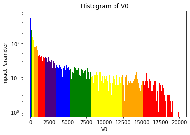
Figure 16. Histogram of v0 distribution according to the event number in logarithmic scale.

We assess the impact parameter of all events and rank the impact parameter from each event in ascending order, making sure that each pair——one impact parameter and its corresponding event number——are still assigned to each other. It works like the index we can use: if we input the event number, the output will be its impact parameter, and vice versa. Since we intend to analyse how the centrality of a collision influences the number of participants, we divide all events into 11 categories based on their ranking in impact parameter: starting with 5% intervals from top 0% to 5%, 5%~10%, and from 10% onwards we take a 10% interval to 20% then to 30% and so on, covering a full spectrum of impact parameter from 0% to 100%. A detailed description can be seen in Figure.16, the horizontal axis refers to the v0 amplitude, and the y-axis refers to the event number (4869 events) in a logarithmic scale.

For each quantile of impact parameter, we select and analyse the first 20 events according to the ranking of the event number, which we consider as a random selection since the event number has no necessary relationship with its corresponding impact parameter. This guarantees the effectiveness and generalizability of the conclusion. Then for each quantile, the \( Δϕ \) and \( Δη \) of each layer (a total of 3 layers) are calculated. After going through all the processes described in the essay in serious order, 33 graphs are generated, and 33 counts are calculated. For each interval of centrality, we combine the three layers (n=3, see Eq.1) and calculate the average of the counts of each layer to get an effective final count.

\( \bar{x}=\frac{1}{n}\sum _{i=1}^{n}{x_{i}} \)

Equation 1. Average count

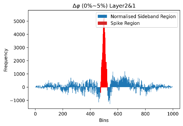
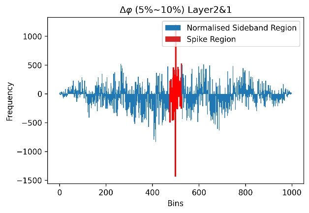
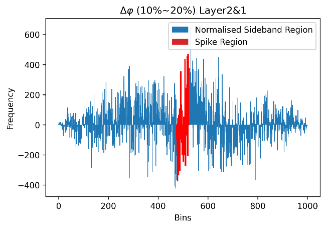
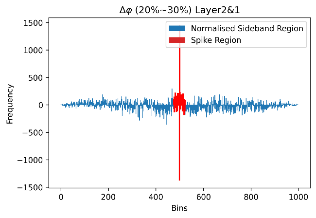
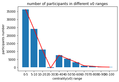
Figure 21. Number of particles produced related to centrality. (Anomaly at centrality 20-30%)

The general pattern can be fitted through a conic curve, and we arrive at the conclusion that: with the increase of the impact parameter, the centrality of collision is smaller, and the number of particles generated by Au+Au collision also decreases nonlinearly. In addition, for those invalid events, after careful analysis of their event number, number of signals detected, and impact parameter, we found out that all 131 invalid events belong to the 0%~5% quantile and all of them have relatively large number of signals detected which can be seen on their headers. Based on this evidence, we reasonably hypothesise that these events surpass the number-of-line limitation and therefore are abandoned by the data collector. Eliminating those events before the analysis might affect the result by slightly reducing the number of sample data from events belonging to 5% which we consider not a big problem due to the already big enough amount.

7. Conclusion

We have implemented the method of finding charged particle multiplicity in various conditions of nuclei overlap Au+Au collisions at S_NN = 200 GeV by working with raw data from ALICE. The reconstruction of the detector geometry allows the pseudorapidity and azimuth to be found and the mechanism of calculating their changes when particles pass through layers allows for the use of the sideband method. Post normalisation results showed promising and consistent count numbers to multiplicity, and the division by centrality helps with understanding how different collisions can contribute differently to particle production. The change in multiplicity with centrality proves that central collisions give more collision products than peripheral collisions and conveys the significance of head-on collisions in future studies at the LHC. Despite the merits, it is worth being aware of the limitations of this method such as the non-uniform distribution of data points when applying the sideband method, as well as the non-ideal results that arose from the negative region produced from signal subtractions. Therefore, the results are considerably evident in presenting a general picture of collision aftermaths, yet the drawbacks of the methods employed does mean it will have to co-exist with a certain degree of robustness.

Acknowledgments

Chensu He, Chia-che Lai, Qixian Jin, and Pengyun Lai contributed equally to this work and should be considered co-first authors.

References

[1]. STAR Collaboration. Measurement of Inclusive Charged-Particle Jet Production in Au+Au Collisions at √ SNN = 200 GeV. Jan. 11AD. Accessed 19 Aug. 2023. https://doi.org/10.1016/j.physletb.2017.04.050. Accessed 19 Aug. 2023.
[2]. “Time Projection Chamber | Alice-Public.web.cern.ch.” Alice.cern, alice.cern/time-projection-chamber. Accessed 19 Aug. 2023.
[3]. Pcharito. “English: Schematics of the ALICE Subdetectors.” Wikimedia Commons, 27 Feb. 2014, commons.wikimedia.org/wiki/File:2012-Aug-02-ALICE_3D_v0_with_Text_(1)_2.jpg. Accessed 19 Aug. 2023.
[4]. Particle identification in ALICE boosts QGP studies CERN Courier, 23 August 2012
[5]. Beolè, S. “The ALICE Inner Tracking System: Performance with Proton and Lead Beams.” Physics Procedia, vol. 37, 2012, pp. 1062–1069, https://doi.org/10.1016/j.phpro.2012.02.443.
[6]. Jales, Allan, and Thomas Gaehtgens. Muon Efficiency Studies Using Tag and Probe Method. Oct. 2020.
[7]. Neutelings, Izaak. CMS Coordinate System. tikz.net/axis3d_cms/.
[8]. Nowakowski, Piotr, et al. “Distributed Simulation and Visualization of the ALICE Detector Magnetic Field.” Computer Physics Communications, vol. 271, Feb. 2022, p. 108206, https://doi.org/10.1016/j.cpc.2021.108206. Accessed 1 May 2022.
[9]. Jales, Allan, and Thomas Gaehtgens. Muon Efficiency Studies Using Tag and Probe Method. Oct. 2020.
[10]. Baudot, Jérôme. ESIPAP 2016 -Module 1 Physics of Particle and Astroparticle Detectors Tracking.
[11]. Basu, Sumit, et al. Multiplicity and Pseudorapidity Density Distributions of Charged Particles Produced in Pp, PA and AA Collisions at RHIC & LHC Energies. 12 Nov. 2020.
Cite this article
He,C.;Lai,C.;Jin,Q.;Lai,P. (2024). Study of charged particle multiplicity with centrality in Au+Au collisions at √SNN = 200 GeV. Theoretical and Natural Science,43,68-79.
Data availability
The datasets used and/or analyzed during the current study will be available from the authors upon reasonable request.
Disclaimer/Publisher's Note
The statements, opinions and data contained in all publications are solely those of the individual author(s) and contributor(s) and not of EWA Publishing and/or the editor(s). EWA Publishing and/or the editor(s) disclaim responsibility for any injury to people or property resulting from any ideas, methods, instructions or products referred to in the content.
About volume
Volume title: Proceedings of the 3rd International Conference on Computing Innovation and Applied Physics
© 2024 by the author(s). Licensee EWA Publishing, Oxford, UK. This article is an open access article distributed under the terms and
conditions of the Creative Commons Attribution (CC BY) license. Authors who
publish this series agree to the following terms:
1. Authors retain copyright and grant the series right of first publication with the work simultaneously licensed under a Creative Commons
Attribution License that allows others to share the work with an acknowledgment of the work's authorship and initial publication in this
series.
2. Authors are able to enter into separate, additional contractual arrangements for the non-exclusive distribution of the series's published
version of the work (e.g., post it to an institutional repository or publish it in a book), with an acknowledgment of its initial
publication in this series.
3. Authors are permitted and encouraged to post their work online (e.g., in institutional repositories or on their website) prior to and
during the submission process, as it can lead to productive exchanges, as well as earlier and greater citation of published work (See
Open access policy for details).