1. Introduction

Calcium imaging is a technique used to observe neuronal activity. It involves labeling calcium ions in neurons using calcium indicators and detecting changes in the fluorescent signal emitted by the indicators.

During neuronal activity, the change of calcium ion concentration is closely related to the electrical activity of neurons. Through calcium indicators, these changes in calcium ion concentration can be translated into changes in the fluorescence signal. Fluorescence microscopes (maikeruoscope) and corresponding imaging systems are used to observe and record these fluorescence signals.

The advantage of calcium imaging is the ability to observe large numbers of neurons simultaneously and to provide spatial and temporal resolution of neuronal activity. This makes calcium imaging a common tool in neuroscience research to study the function of neural circuits, the interactions between neurons, and the activity of the nervous system during different behavioral and cognitive processes.[1]

Calcium imaging analysis is a very complete technology, it includes many steps, such as how to inject calcium indicators, how to extract signals, and data analysis, etc. We only studied a part of it

We have developed a strong calculation method that can be used to analyze GCaMP fluorescent data. GCaMP is a causal coding calcium indicator, the most widely used is to observe the activity of thousands of neural groups at the same time using modern fluor imaging techniques.

We use some background knowledge of basic information processing, statistical inference, hypothesis testing and basic principles of graph theory. We should use these principles to help interpret the primary GCaMP fluorescence data recorded from the waking rats.

Our initial data were two GCaMP6(special edition of GCaMP) fluorescent data sets containing temporal sequence traces of hundreds of rats primary visual cortex (V1) elements. These elements are located in a three-dimensional volume of about 800 μm x 800 μm x 100 μm. The axial depth is limited by various physical limits. This volume contains a large part of two-thirds of the layers, and many of the higher layers of the large brain are born in the skin.

The GCaMP fluorescent record sample is made as the phase pair modification of the fluorescent phase to the basic fluorescent water level for each celestial element n and each time point m

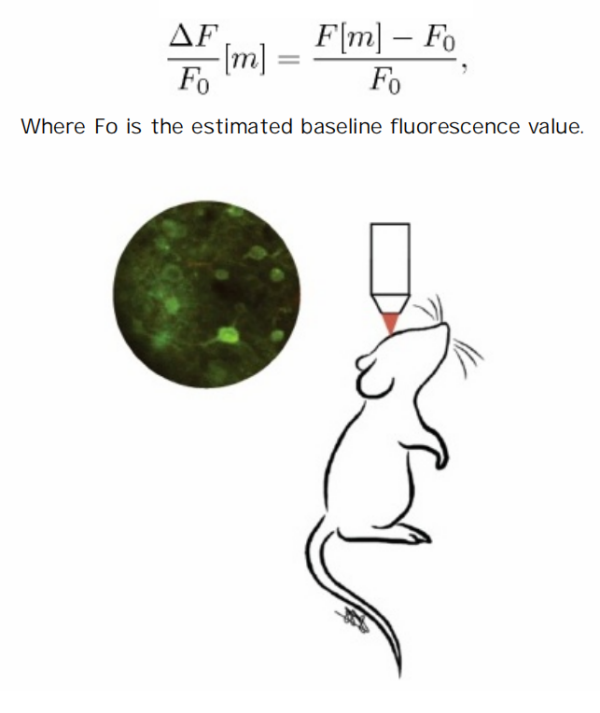
Figure 1. The original data is derived from experimental mice

2. Related work

Calcium imaging, especially using genetically encoded calcium indicators like GCaMP, has become a key method for observing neural activity [2]. Over the years, various methods have been developed and optimized to analyze GCaMP fluorescence data.[3]

Tian et al made significant advancements in improving the GCaMP indicator for observing neural activity in worms, fruit flies, and mice. [4] Their research emphasized the importance of optimizing the sensitivity of GCaMP indicators, highlighting the evolving nature of these tools and their potential to capture neural dynamics in different organisms.

Chen et al highlighted the challenges of threshold fluorescence modes. They laid down fundamental concepts in the field of using GCaMP for neuronal activity imaging. [5] This method, although powerful, often faces challenges distinguishing high-frequency changes from actual neural activity, emphasizing the importance of robust analytical techniques.

In the exploration of optimizing calcium imaging, Dana et al delved deeply into high-performance calcium sensors for imaging neural activity.[6] Their work centered on creating more sensitive and faster variants of GCaMP, elucidating the need for a balance between sensitivity and noise.

There are many ways to analyze calcium imaging data. One of the most notable methods is a toolkit called “EZcalicu”[7]. This toolkit is convenient as it produces results directly. However, EZcalicu has its limitations. Specifically, it only supports the analysis of .tiff files. Data formats like .AVI or .mat are incompatible. Given the frequent challenges of converting complex data formats to either .TIFF or .AVI, this posed a significant limitation. Recognizing this challenge, we embarked on the task of developing our own set of codes specifically tailored for similar data analysis, using . MAT data as an example.

Moreover, the work of Eftychios Pnevmatikakis on the MATLAB toolbox, despite being commendable, also has its limitations. While it can efficiently analyze calcium imaging data, it often blurs high-frequency changes, potentially losing key information.

Our approach is largely influenced by the aforementioned research, and we have integrated various elements from them. However, our goal is to address some of these limitations, especially when it comes to preserving high-frequency data without compromises. We adopted a combination of high-pass filtering, Gaussian mixture modeling, and connectivity centrality, ensuring a comprehensive analysis of GCaMP fluorescence data.

3. Research methods

Our workflow is shown in the figure 2

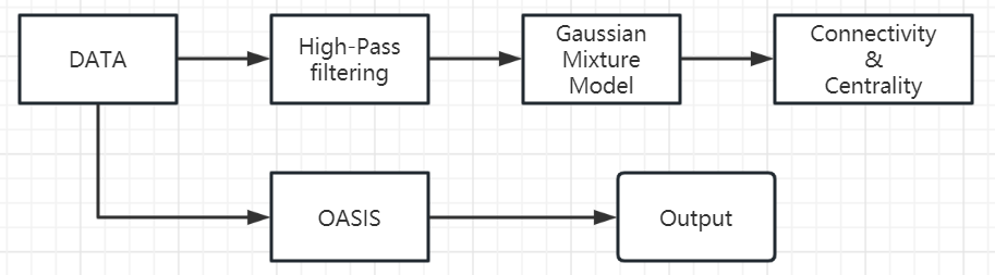
Figure 2. Flow chat

3.1. Filtration

Low frequency base line drift is present in each time sequence track due to motion, image noise, and/or optical bleaching. We are interested in the relative high frequency variation of GCaMP. High frequency variation is the result of calcium inflow and outflow, and is related to the direct discharge of neurons.

We must design a suitable high-pass filter and the filter should be used in tandem data to eliminate the above low frequency drift in each record of the Scriptures. We must ensure that, when designing the filter, only the unwanted low frequency drift induced by the above mentioned error is eliminated and the calcium inflow and outflow fluorescence changes are retained.

First we draw the mean Fourier amplitude spectrum and determine an appropriate cut-off frequency for the logical high pass filter that applies to all GCaMP time sequence traces.[8]

In the frequency domain, the ideal high-pass filter is defined, for some cutoff frequency ωc, as follow

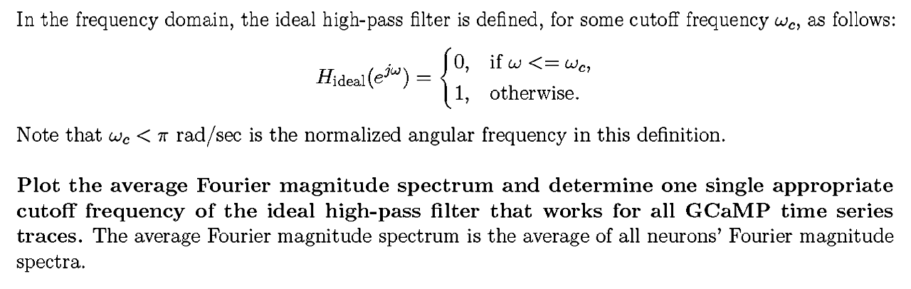
After analysis and calculation, we determined that ωc = 0.198

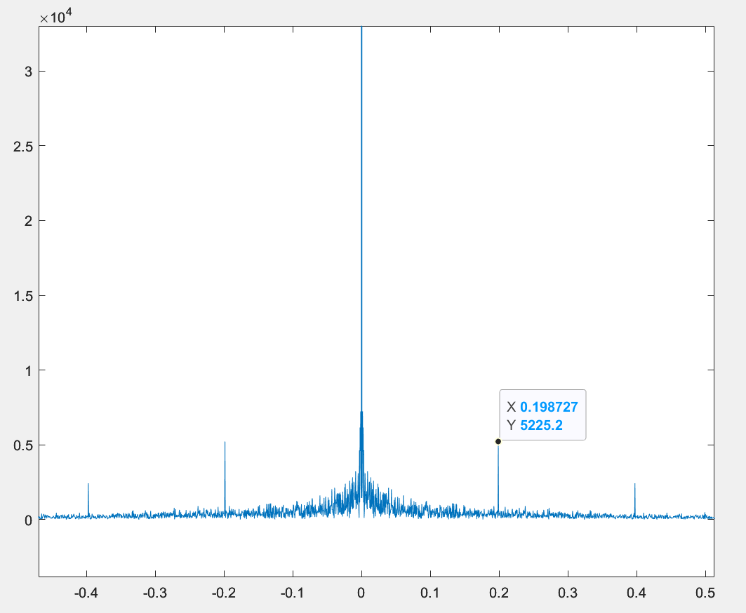
Figure 3. A histogram showcasing the distribution of fluorescence intensities in the collected data

Then we get the raw data and the filter coefficient. Then we can filter the raw data in the time domain resorts to convolving the data with the filter coefficients in the time domain. The result we get after the convolution should the filtered data.

We use Matlab to achieve, the code is as follows

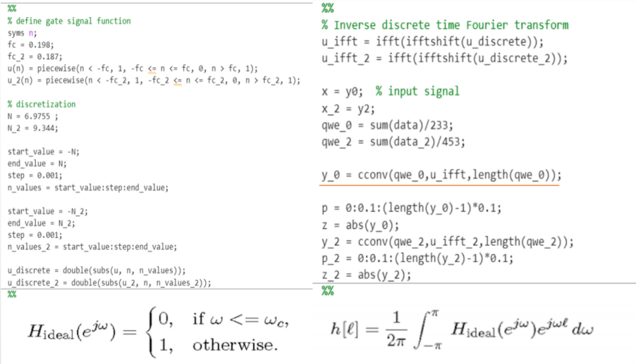
Figure 4. Defining and Processing Discrete-Time Fourier Transform with Ideal Gate Signal

And next we did Filtering by convolution:

we using convolution. Filtering data in the time domain resorts to convolving the data with the filter coefficients in the time domain. We design this code

y_0 = cconv(qwe_0,u_ifft, length (qwe_0))

(What this expression means is to convolve qwe_0 and u_ifft cyclically and store the result in y_0. length(qwe_0) is used to specify the length of the convolution, which is the same length as qwe_0.) Our results are shown in the figure 2 and 3 below

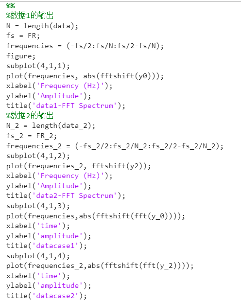
Figure 5. Code Spectral Analysis of Frequency and Time Domain Using Fast Fourier Transform

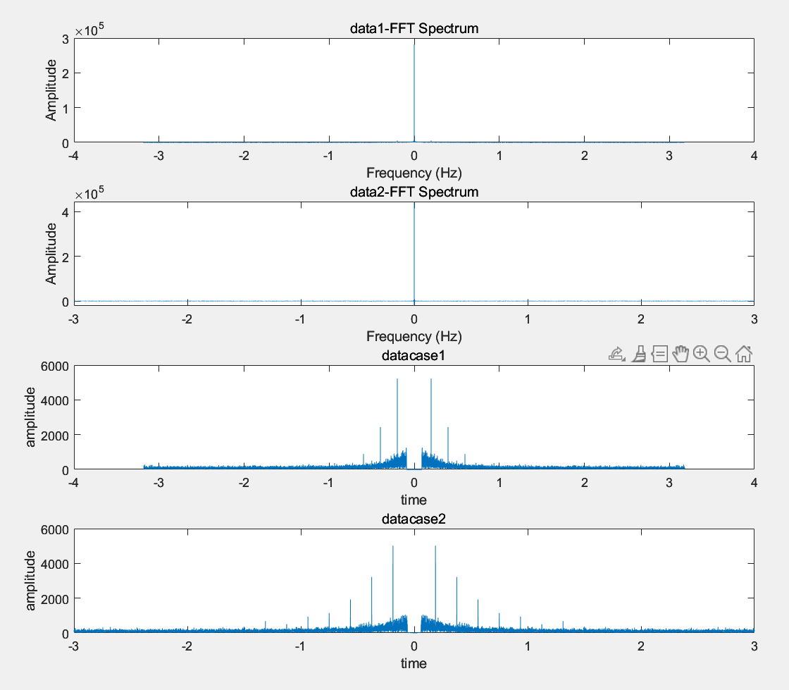
Figure 6. Result 1 Visualization of the Gaussian mixture model’s ability to differentiate neuronal states.

3.2. About the Gaussian mixture model

The function of Gaussian mixture model fitting is to model and analyze the activity data of neurons. In our project, Gaussian mixture model is used to fit neuronal data after high-pass filtering. The specific steps are as follows: First, the neuron data after high-pass filtering is taken as a sample, assuming that the sample of each neuron is generated by a Gaussian mixture model with two mixed components. One of the mixed components represents the baseline state and the other represents the excited state.Then, using built-in functions or packages in Python or MATLAB, a Gaussian mixture model is fitted to a sample of each neuron. The goal of fitting is to find the best model parameters so that the model can best describe the sample data. By fitting the Gaussian mixture model, the probability density function of each neuron can be obtained, so that the activity pattern and interaction of neurons can be better understood. These probability density functions can be used for further analysis, such as calculating correlations between neurons, exploring connectivity and centrality between neurons, etc. Therefore, Gaussian mixture model fitting plays an important role in studying neuronal activity and the function and structure of neural networks.

But because of time and schedule, the work is still being done.

3.3. OASIS

OASIS (Open Source Imaging Spike Sorting) is a MATLAB toolkit for offline analysis and peak detection of neural activity. [9] It provides a set of functions and tools for processing and analyzing calcium imaging data.

The main features of OASIS-MATLAB include: Data preprocessing, Peak detection, Data analysis, Utility functions.

So, how does the OASIS filter the signal?

Initialization: Firstly, the signal needs to be initialized.

Attenuation Rate Estimation: Next, OASIS distinguishes the desired signal component from the noise component by estimating the attenuation rates of the signal. [10]

Filtering Iterations: In each iteration, OASIS filters the signal based on the estimated attenuation rates.

Convergence Check: After each iteration, OASIS examines the difference between the filtered result and the previous iteration.

Then we using “deconvolveCa” to perform deconvolution analysis on the original calcium imaging data. (code as follow)

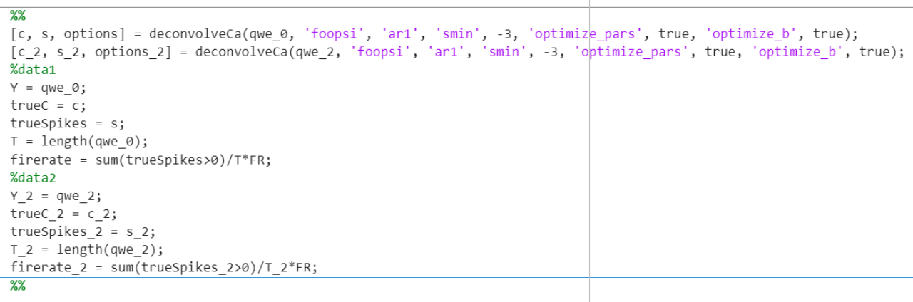
Figure 7. Code representation of the estimated neural activity and estimated calcium indicator concentration using the deconvolution algorithm

“c”- the estimated neural activity trace

“s” - the estimated calcium indicator concentration signal

“options” - a structure that contains parameter options for configuring the deconvolution algorithm.

This is a cyclic convolution calculation in signal processing that we designed. The deconvolveCa function is used in the code for signal deconvolution operations.

First, the code deconvolveCa deconvolved the signal qwe_0 by calling the deconvolveca function, and assigned the returned results to the variables c, s, and options, respectively. Similarly, the code performs a convolution operation on the signal qwe_2 and assigns the result to the variables c_2, s_2, and options_2.

Then, we define some variables and calculations. Y and Y_2 represent signals qwe_0 and qwe_2, respectively. truec and trueC_2 represent the result c and c_2 after deconvolution, respectively. truespikes and truespikes_2 represent the result s and s_2 after deconvolution, respectively. T and T_2 represent the length of the signal, and firerate_2 represent the frequency of the pulse in the result after deconvolution, respectively.

Next we will plot the result using Matlab. Here is an explanation of our code: First, the code initializes the graph by setting the paper size of the graph to ‘[15, 2.5]’ and calling the ‘init_fig’ function. Next, use the ‘hold on’ command to keep what is already on the graph and allow multiple graphs to be drawn on the same graph. Then, the color variable ‘col’ is defined, which contains the RGB values for the three colors. Next, plot the fluorescence tracing curve using the ‘plot’ function. ‘(1:T)/FR’ represents the time point on the X-axis, and ‘Y(1,:)’ represents the corresponding fluorescence value. The ‘o’ parameter is used to specify the color, and the ‘uint8(col(2))’ is used here for the second color. Then, plot the calcium ion trace curve using the ‘plot’ function. ‘(1:T)/FR’ represents the time point on the X-axis, and ‘trueC(:,1)’ represents the corresponding calcium ion value. The ‘color’ parameter is used to specify the color, here ‘k’ is used for black. Next, use the ‘find’ function to find the point in time when the pulse occurred, and use the ‘plot’ function to plot the location where the pulse occurred. ‘[1,1]*tsp(m)/FR’ represents the point in time at which the pulse occurs, and ‘[0, 1]’ represents the starting and ending positions on the Y-axis. The ‘color’ argument is used to specify the color, and uint8(col(3)) is used here to represent the third color. Then, use the ‘axis tight’ command to fit the axes to the data range. Next, use ‘xlabel’ and ‘ylabel’ to set the labels for the x and y axes, respectively. Then, a legend is drawn using the ‘Legend’ function, where ‘y’, ‘c’, and ‘s’ represent fluorescence tracking, calcium ion tracking, and pulse generation, respectively. Finally, use the ‘set’ function to set the properties of the current graph object, where ‘fontweight’ is set to ‘bold’. (figure 5)

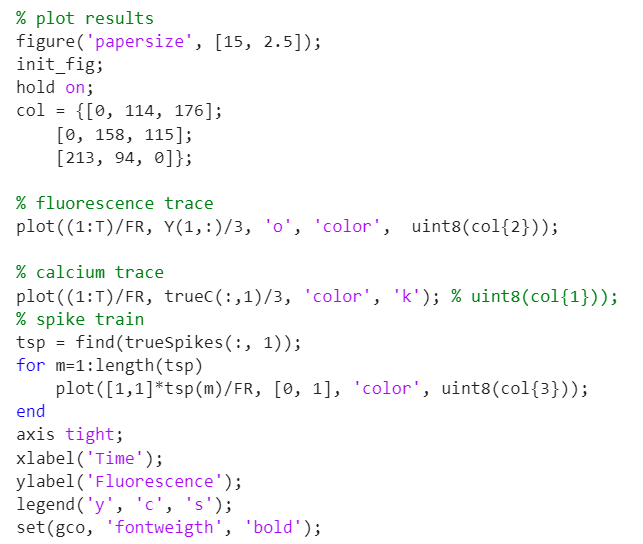
Figure 8. Plotting Fluorescence Trace, Calcium Signal Trace, and Spike Event Time Series

Need attention that Fire rate refers to the frequency at which a neuron generates action potentials, also known as spikes, within a certain period of time.

0.4300 is fire rate of datecase1 and 0.7401 is fire rate of datecase2

Our result is shown in Figure 6

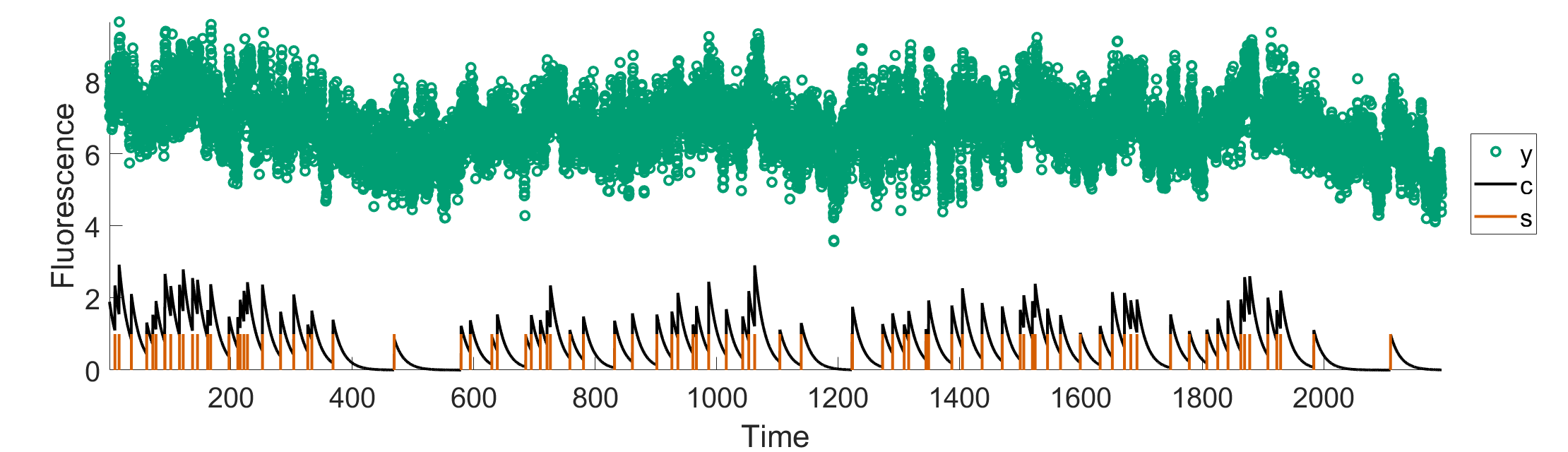
Figure 9. Comprehensive graph showcasing fluorescence trace, calcium trace, and spike train.

“Y”- flourecence trace

“c” - calcium trace

“s”- spike train

Next we define a few variables and create two empty 2D arrays using the zeros function. We store the randomData value of each data point into a 2D array for subsequent analysis and processing (possible uses include statistical analysis, graph drawing, model training, etc.)

3.4. Connectivity & Centrality

The work of this step is to calculate the correlation coefficient matrix R from the standardized data for each dataset. Now that we have processed and standardized the GCaMP fluorescence time series data for each neuron imaging in each dataset, we can begin to examine the paired interactions between all neurons in the population. The correlation coefficient describes how similar the activity of one neuron is to that of another. Thus, correlation coefficients provide a very simple and easy way to glimpse the connectivity of neural populations. The number of neurons in data 1 and data 2 is 233 and 453, respectively

So we need to get a coefficient matrix 233 by 233 and a matrix 453 by 45

Here are our results (figure 10)

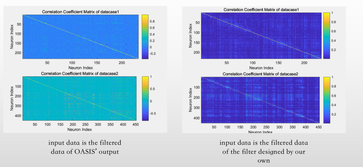
Figure 10. Correlation matrices of the analyzed neuronal populations, indicating the connectivity between different neurons.

4. Conclusion and prospect

Our aim was to explore how GCaMP fluorescence data can be analyzed using computational methods to better understand the patterns and interactions of neuronal activity. By calculating the correlation coefficient matrix between neurons, we can understand the interactions and connections between neurons, and further reveal the structure and function of neural networks. At the same time, the use of high-pass filters can help us eliminate noise and drift, extract the high-frequency changes associated with neuronal activity, and thus more accurately study the behavior of neurons. We use Matlab as our primary tool, along with the application of principles such as basic signal processing, statistical inference, hypothesis testing, and graph theory, to help understand raw GCaMP fluorescence data recorded from awake, behavioral mice. The results have important implications for understanding the patterns and interactions of neuronal activity.

What else can we expand?

Gaussian Mixture Model:

When we need to analyze a set of data, the Gaussian mixture model (GMM) can help us better understand the distribution of the data. In this case, we can better distinguish between the resting state and the activated state.

Design a better filter:[11]

Since our filter can only filter the low frequencies signals, so the effect of filtering is not very good. We can design a better filter which can also filter the overfrequences.

Acknowledgements

I would like to express my deepest gratitude to everyone who has supported and assisted me throughout the completion of this paper.

First and foremost, I would like to thank my supervisor, Professor Liu Chunlei. Thank you for your invaluable guidance and selfless support. Your vast knowledge and profound academic expertise have been instrumental in driving my research work. Your patient guidance and valuable advice have helped me overcome challenges and constantly improve.

I would also like to express my thanks to Mr. Yuan Ye, the teaching assistant. Your explanations and tutoring in the classroom have helped me understand and grasp many important concepts and skills. Your patience and meticulousness have made me feel warmth and support in my learning journey.

Furthermore, I want to thank my teammate, Felix. We have collaborated closely in our research project, working together to solve problems and overcome difficulties. Your wisdom and creativity have brought many new ideas and breakthroughs to our research work. Thank you for your teamwork spirit and selfless dedication.

Lastly, I want to express my gratitude to all the teachers from CIS. Your teachings and guidance have been immensely beneficial to me. Your vast knowledge and professional experience have provided me with a broad academic perspective and inspiration. Thank you for your care and support.

Once again, I extend my heartfelt appreciation to everyone who has supported and assisted me. Without your support and encouragement, I would not have been able to complete this project. Thank you all!

References

[1]. Zhang, Y., Rózsa, M., Liang, Y. et al. Fast and sensitive GCaMP calcium indicators for imaging neural populations. Nature 615, 884–891 (2023). https://doi.org/10.1038/s41586-023-05828-9
[2]. Shemesh, O., Linghu, C., Piatkevich, K. D., Goodwin, D. R., Gritton, H., Romano, M. F., ... & Boyden, E. (2020). Precision Calcium Imaging of Dense Neural Populations via a Cell-Body-Targeted Calcium Indicator. Neuron. Available at: https://www.cell.com/neuron/pdf/S0896-6273(20)30398-6.pdf
[3]. Dorostkar, M., Dreosti, E., Odermatt, B., & Lagnado, L. (2010). Computational processing of optical measurements of neuronal and synaptic activity in networks. Journal of Neuroscience Methods. Available at: https://www.sciencedirect.com/science/article/pii/ S0165027010000725
[4]. Tian, L., et al. (2009). Imaging neural activity in worms, flies and mice with improved GCaMP calcium indicators. Nature Methods, 6(12), 875–881.
[5]. Chen, T. W., et al. (2013). Ultrasensitive fluorescent proteins for imaging neuronal activity. Nature, 499(7458), 295–300.
[6]. Dana, H. et al. (2019). High-performance calcium sensors for imaging activity in neuronal populations and microcompartments. Nature Methods, 16(7), 649-657.
[7]. Cantu, D. A., Wang, B., Gongwer, M. W., He, C. X., Goel, A., Suresh, A., Kourdougli, N., Arroyo, E. D., Zeiger, W., & Portera-Cailliau, C. (2020). EZcalcium: Open-Source Toolbox for Analysis of Calcium Imaging Data. Technology and Code, doi: 10.3389/fncir.2020.00025.
[8]. M. T. Valley,* M. G. Moore,* J. Zhuang, N. Mesa, D. Castelli, D. Sullivan, M. Reimers, and J. Waters 17 JAN 2020https://doi.org/10.1152/jn.00304.2019
[9]. Pachitariu, M., Steinmetz, N. A., Kadir, S. N., Carandini, M., & Harris, K. D. (2016). Fast and accurate spike sorting of high-channel count probes with KiloSort. Advances in Neural Information Processing Systems, 29.
[10]. Front. Mol. Neurosci., 05 December 2014 Sec. Methods and Model Organisms Volume 7 - 2014 | https://doi.org/10.3389/fnmol.2014.00097
[11]. Stopper, G., Caudal, L.C., Rieder, P. et al. Novel algorithms for improved detection and analysis of fluorescent signal fluctuations. Pflugers Arch - Eur J Physiol 475, 1283–1300 (2023). https://doi.org/10.1007/s00424-023-02855-3
Cite this article
Qin,H. (2024). Computational analysis of GCaMP fluorescence data in neuronal activity. Theoretical and Natural Science,46,163-172.
Data availability
The datasets used and/or analyzed during the current study will be available from the authors upon reasonable request.
Disclaimer/Publisher's Note
The statements, opinions and data contained in all publications are solely those of the individual author(s) and contributor(s) and not of EWA Publishing and/or the editor(s). EWA Publishing and/or the editor(s) disclaim responsibility for any injury to people or property resulting from any ideas, methods, instructions or products referred to in the content.
About volume
Volume title: Proceedings of the 2nd International Conference on Modern Medicine and Global Health
© 2024 by the author(s). Licensee EWA Publishing, Oxford, UK. This article is an open access article distributed under the terms and
conditions of the Creative Commons Attribution (CC BY) license. Authors who
publish this series agree to the following terms:
1. Authors retain copyright and grant the series right of first publication with the work simultaneously licensed under a Creative Commons
Attribution License that allows others to share the work with an acknowledgment of the work's authorship and initial publication in this
series.
2. Authors are able to enter into separate, additional contractual arrangements for the non-exclusive distribution of the series's published
version of the work (e.g., post it to an institutional repository or publish it in a book), with an acknowledgment of its initial
publication in this series.
3. Authors are permitted and encouraged to post their work online (e.g., in institutional repositories or on their website) prior to and
during the submission process, as it can lead to productive exchanges, as well as earlier and greater citation of published work (See
Open access policy for details).