1 Introduction

The Fourier Transform is a critical mathematical method with extensive applications in quantum mechanics [1]. Converting functions from the temporal or spatial domain to the frequency domain enables the comprehension and analysis of wave functions' behavior. This article explores the applications of this tool in quantum mechanics, focusing on key theorems and principles such as the Uncertainty Principle, the Planck-Einstein relation, Parseval's identity, and the Fourier Transform solution of the Schrödinger equation. These foundational elements highlight the theoretical importance of the Fourier Transform in the study and application of quantum mechanics.

Quantum mechanics, one of the most revolutionary scientific advancements of the 20th century, is a fundamental theory that explains the behavior of nature on the scale of both atomic and subatomic in physics [2]. The heart part of quantum mechanics is the wave function, providing a probability distribution for the position and momentum of particles. The Fourier Transform is particularly valuable in this context because it allows for the transformation of wave functions between the time/spatial domain and the frequency (or momentum) domain, thereby providing critical insights into the behavior and characteristics of quantum systems.

In the past five years, the application of Fourier Transforms in quantum mechanics has seen significant advancements. Researchers have developed more efficient algorithms for performing Fourier Transforms on quantum computers, which has opened new possibilities for simulating quantum systems. These advancements have led to more accurate and faster simulations of complex quantum phenomena, such as quantum entanglement and decoherence.

Moreover, the integration of Fourier Transform techniques with machine learning has enabled the prediction and analysis of quantum system behaviors with unprecedented precision. This hybrid approach has been particularly successful in studying time-dependent quantum systems, where the dynamics can be captured and analyzed more effectively using Fourier-based methods.

In the subsequent sections of this article, this paper will delve deeper into the specific applications and implications of the Fourier Transform in quantum mechanics. This paper will start by discussing the theoretical underpinnings and mathematical properties of the Fourier Transform, including its linearity, shift, and scaling properties. Following this, this paper will explore the Plancherel theorem and Parseval's identity, highlighting their importance in preserving energy and inner products in quantum systems.

Next, this paper will examine the Heisenberg Uncertainty Principle in detail, demonstrating how the Fourier Transform provides a mathematical framework for understanding the trade-offs between position and momentum uncertainties. This paper will also discuss the Planck-Einstein relation and its relevance to the energy distribution of quantum states, using Fourier analysis to elucidate these relationships.

Finally, this paper will present case studies and examples of how the Fourier Transform is utilized to solve the Schrödinger equation in different quantum mechanical scenarios. These examples will illustrate the practical applications of Fourier analysis in simplifying and solving complex quantum problems, reinforcing the transformative impact of this mathematical tool on the field of quantum mechanics.

2 Methods and Theory

2.1 Fourier Transform

This article centers on the use of Fourier transforms to prove or solve theorems or problems within quantum mechanics. The main method of this article is Fourier transform [3]

\( \hat{f}(t)=\int_{R}^{} f(x)e^{-2πix}dx,\ \ \ （1） \)

where \( \hat{f}(t) \) is called the Fourier function of \( f(x) \) . The first linear property means that if there are two signals \( f(t) \) and \( g(t \) ), and their respective Fourier transforms are \( F(ω) \) and \( G(ω) \) , then the Fourier transforms satisfy the following relationship for any two invariants m and n:

\( mF(ω)+nG(ω)=F[mf(t)+ng(t)],mF(ω)+nG(ω)=F[mf(t)+ng(t)]\ \ \ （2） \)

This means that the Fourier transform can be performed on \( f(t) \) and \( g(t) \) separately, and then the results can be summed up to give the same result as if the Fourier transform were performed directly on \( mf(t)+ng(t). \)

If the Fourier transform of \( f(t) \) is \( F(ω) \) , then the Fourier transform of \( f(t-t_{0}) \) (i.e., \( f(t) \) is shifted to the right by \( t_{0} \) in the time domain) is: \( e^{-jωt_{0}}F(ω)) \) . This indicates that a time domain shift leads to a phase factor in the frequency domain. If the Fourier transform of \( f(t) \) is \( F(ω), \) then the Fourier transform of \( f(at) \) (i.e., the scaling of \( f(t \) ) by a factor of a in the time domain) is

\( F =\frac{1}{|a|}F(\frac{ω}{a})\ \ \ （3） \)

which demonstrates that scaling in the time domain results in alterations to both scaling and magnitude in the frequency domain.

The symmetry properties of the Fourier transform include the symmetry of the real and imaginary parts. If \( f(t) \) is a real function, then the real part of its Fourier transform \( F(ω) \) is an even function, and the imaginary part is an odd function:

\( Re[F(-ω)]=Re[F(ω)]\ \ \ （4） \)

\( Im[F(-ω)]=-Im[F(ω)]\ \ \ （5） \)

Furthermore, if \( f(t) \) is a real function, then the Fourier transform \( F(ω) \) of \( f(t) \) satisfies the following relation:

\( F(-ω)=F*(ω)\ \ \ （6） \)

where \( F*(ω) \) is the complex conjugate of \( F \) (ω), which indicates that the Fourier transform of \( f(t) \) is conjugate symmetric.

2.2 Plancherel Theorem and Parseval's Identity

Plancherel Theorem and Parseval's identity are fundamental results in Fourier analysis that are crucial for energy and inner product preservation in quantum mechanics [4].

The Plancherel theorem states that for any function \( f∈L^{2}(R^{n}), \) its Fourier transform \( \hat{f}∈L^{2}(R^{n}) \) , and the following equality holds:

\( \int_{R^{n}}^{} |f(x)|^{2} dx=\int_{R^{n}}^{} |\hat{f}(k)|^{2} dk\ \ \ (7) \)

Parseval's identity states that for any functions \( (f,g∈L^{2}(R^{n})) \) , the inner product is preserved under the Fourier transform:

\( \int_{R^{n}}^{} f(x)\overline{g(x)} dx=\int_{R^{n}}^{} \hat{f}(k)\overline{\hat{g}(k)} dk\ \ \ （8） \)

This shows that the Fourier transform preserves the inner product in the \( L^{2} \) space, demonstrating its importance in quantum mechanics. These theorems underline the fundamental properties of the Fourier transform, ensuring energy conservation and inner product preservation, which are crucial for quantum mechanical systems.

2.3 Heisenberg Uncertainty Principle

Heisenberg's uncertainty principle explains the relationship between the uncertainty in a particle's position and momentum. [5]:

\( Δx⋅Δp≥\frac{ℏ}{2}\ \ \ （9） \)

where \( Δx \) represents the uncertainty of the position, \( Δp \) denotes the uncertainty in the momentum, and \( ℏ \) is the approximate Planck constant.

In quantum mechanics, a particle's state is described by the wave function \( ψ(x \) ), This wave function represents the probability amplitude of locating the particle at a specific position x. Essentially, \( ψ(x \) ) provides a mathematical description of the likelihood of finding the particle at various positions in space. [6].

The Fourier function \( ϕ(p) \) of wave function \( φ(x) \) describes the probability amplitude of the particle's momentum space

\( ϕ(p)=\frac{1}{\sqrt[]{2πℏ}}\int_{R}^{} φ(x)e^{-\frac{ipx}{ℏ}}dx\ \ \ （10） \)

inverse transform as

\( φ(x)=\frac{1}{\sqrt[]{2πℏ}}\int_{R}^{} ϕ(p)e^{\frac{ipx}{ℏ}}dp.\ \ \ （11） \)

Uncertainty of position \( Δx \) and momentum \( Δp \) is defined as the standard deviation of wave function \( ψ(x) \) and \( ϕ(p): \)

\( (Δx)^{2}=⟨x^{2}⟩-⟨x⟩^{2}\ \ \ （12） \)

\( (Δp)^{2}=⟨p^{2}⟩-⟨p⟩^{2}\ \ \ （13） \)

According to the nature of the Fourier transform, the wave function has a certain duality between the time and frequency domains (momentum space). Specifically, the width of the wave function is inversely related to the width of its Fourier transform. Suppose that \( φ(x) \) and \( ϕ(p) \) satisfied the normalizing conditions:

\( \int_{-∞}^{∞} |φ(x)|^{2}dx=1,\int_{-∞}^{∞} |ϕ(p)|^{2}dx=1\ \ \ （14） \)

Applying the Cauchy-Schwarz inequality [7], and by conducting norm analysis on ε (x) and ε (p), the following relationship is obtained:

\( Δx⋅Δp≥\frac{ℏ}{2}\ \ \ （9） \)

The Fourier transform played the role of a bridge in proving Heisenberg's inequality, through which two interrelated physical quantities, position, and momentum, could be mathematically linked, thus revealing the fundamental uncertainty principle in quantum mechanics.

Using Parseval's identity, this paper can demonstrate the preservation of inner products in position and momentum space, which directly relates to the uncertainty principle. Parseval's identity states that for any wave functions \( ψ(x) \) and \( ϕ(x), \) their Fourier transforms \( (\hat{ψ}(p)) \) and \( (\hat{ϕ}(p)) \) satisfy:

\( \int_{R}^{} ψ(x)\overline{ϕ(x)} dx=\int_{R}^{} \hat{ψ}(p)\overline{\hat{ϕ}(p)} dp\ \ \ （15） \)

This implies that the inner product of wave functions is preserved under Fourier transform, ensuring that the probability distributions in position and momentum space are related by:

\( \int_{R}^{} |ψ(x)|^{2} dx=\int_{R}^{} |\hat{ψ}(p)|^{2} dp\ \ \ （16） \)

This equality supports the Heisenberg uncertainty principle by linking the spread (or uncertainty) in position space to the spread in momentum space.

2.4 Planck-Einstein Relation

The Planck Einstein relationship mainly describes the relationship between the energy of photons and their frequency [8]:

\( E=hυ\ \ \ （17） \)

Among them, \( E \) is the energy of the photon, \( h \) is the Planck constant, and \( υ \) is the frequency of the photon.

The state of particles (including photons) is defined by the wave function \( ψ(x,t) \) )In quantum mechanics. [9]. This wave function provides a complete description of the quantum state, encapsulating all the information about the particle's position and momentum probabilities at any given time. The Fourier transform enables the conversion of the wave function from the time domain to the frequency domain, thus revealing its frequency components. Assuming that the wave function \( ψ(x,t) \) can be represented by Fourier transform as:

\( ψ(x,t)=\int_{R}^{} \widetilde{ψ}(k,ω)e^{i(kx-ωt)}dx\ \ \ （18） \)

Among them, \( \widetilde{ψ}(k,ω) \) is the representation of the wave function in the frequency domain (or wavenumber domain), \( k \) is the wavenumber, and \( ω \) is the angular frequency.

According to the Planck Einstein relationship, the relationship between energy \( E \) and frequency \( υ \) can be written as [10]:

\( E=hυ=ℏω\ \ \ （19） \)

where \( ω= 2πυ \) . The Fourier transform is a powerful tool that can help to understand the distribution of wave functions at different frequencies (or energies). For example, suppose the representation of the wave function in the time domain is \( ψ(t) \) . By applying the Fourier transform to \( ψ(t) \) , then obtain \( \widetilde{ψ}(ω \) ), which represents the distribution of the wave function in the frequency domain (or energy domain):

\( \widetilde{ψ}(ω)=\frac{1}{\sqrt[]{2π}}\int_{R}^{} ψ(t)e^{-iωt}dt\ \ \ （20） \)

By analyzing \( \widetilde{ψ}(ω) \) , the contribution of the wave function at different energies (or frequencies) can be obtained.

The Fourier transform can help to understand the relationship between the wave function in the time and frequency (or energy) domains, thus revealing the energy distribution and frequency characteristics of particles (including photons)

2.5 Solution of The Schrödinger Equation

The Fourier transform is crucial for solving the Schrödinger equation, which characterizes the evolution of a particle's wave function in quantum mechanics over time and space. This fundamental equation describes how the quantum state of a physical system changes over time, providing a comprehensive framework for predicting the behavior of particles.

By applying the Fourier transform to the Schrödinger equation, the problem is converted from the spatiotemporal domain to the frequency (or wavenumber) domain. This transformation simplifies the solving process by breaking down complex wave functions into their constituent frequency components. In the frequency domain, differential equations often become algebraic equations, which are generally easier to solve. This method allows for more straightforward analysis and interpretation of the wave function's behavior.

The Schrödinger equation for a non relativistic single particle is typically written as:

\( iℏ\frac{∂ψ(x,t)}{∂t}=-\frac{ℏ^{2}}{2m}\frac{∂^{2}ψ(x,t)}{∂x^{2}}+V(x)ψ(x,t)\ \ \ （21） \)

where, \( ψ(x,t) \) is wave function; \( i \) is an imaginary unit; \( ℏ \) is the reduced Planck constant; m is the mass of the particle; \( V(x) \) is the potential energy function. After performing a Fourier transform on the wave function \( ψ(x,t) \) , the spatial derivative term \( \frac{∂^{2}ψ(x,t)}{∂x^{2}} \) is transformed into:

\( \frac{∂^{2}ψ(x,t)}{∂x^{2}}=\frac{1}{\sqrt[]{2π}}\int_{R}^{} -k^{2\widetilde{ψ}(k,t)}e^{-ikx}dx\ \ \ （22） \)

In this way, the spatial derivative term in the Schrödinger equation is transformed into a form in the wavenumber domain.

Perform Fourier transform on the entire Schrödinger equation to obtain the Schrödinger equation in the wavenumber domain:

\( iℏ\frac{∂\widetilde{ψ}(k,t)}{∂t}=\frac{ℏ^{2}k^{2}}{2m}\widetilde{ψ}(k,t)+\frac{1}{\sqrt[]{2π}}\int_{R}^{} V(x)ψ(x,t)e^{-ikx}dx\ \ \ （23） \)

For different forms of potential energy \( V(x), \) the Fourier transformed Schrödinger equation may be easier to solve. For example, for a free particle (i.e. \( V(x)=0 \) ), the Fourier transformed Schrödinger equation becomes:

\( iℏ\frac{∂\widetilde{ψ}(k,t)}{∂t}=\frac{ℏ^{2}k^{2}}{2m}\widetilde{ψ}(k,t)\ \ \ （24） \)

This equation is a simple linear differential equation that can be solved using standard methods:

\( \widetilde{ψ}(k,t)=\widetilde{ψ}(k,0)e^{-\frac{ℏ^{2}k^{2}}{2m}t}\ \ \ （25） \)

By solving the Schrödinger equation after Fourier transform to obtain k, and then returning to the spacetime domain through inverse Fourier transform to obtain the wave function \( ψ(x,t) \)

\( ψ(x,t)=\frac{1}{\sqrt[]{2π}}\int_{R}^{} \widetilde{ψ}(k,t)e^{ikx}dk\ \ \ （26） \)

This transformation makes the spatial derivative term easier to handle, particularly for specific forms of potential energy functions, and can significantly simplify the solution process. The use of the Fourier transform and its inverse enables flexible conversion between different domains, thereby allowing for more effective analysis and problem-solving in quantum mechanics.

3 Results and Application

3.1 Application of Uncertainty Principle:

Consider a Gaussian wave packet defined in position space as [11]:

\( ψ(x)=(\frac{1}{2πσ_{x}^{2}})^{1/4}e^{-\frac{x^{2}}{4σ_{x}^{2}}}\ \ \ （27） \)

The Fourier transform of this wave packet gives its representation in momentum space:

\( ϕ(p)=\frac{1}{\sqrt[]{2πℏ}}\int_{R}^{} ψ(x)e^{-\frac{ipx}{ℏ}} dx\ \ \ （28） \)

For a Gaussian wave packet, the Fourier transform is also a Gaussian:

\( ϕ(p)=(\frac{σ_{x}^{2}}{ℏ^{2}})^{1/4}e^{-\frac{p^{2}σ_{x}^{2}}{ℏ^{2}}}\ \ \ （29） \)

This shows that a Gaussian wave packet in position space remains Gaussian in momentum space, but with a different width parameter.

For the Gaussian wave packet \( ψ(x), \) the position uncertainty \( Δx \) is given by the standard deviation: \( Δx=σ_{x} \) . For the Gaussian wave packet's Fourier transform \( ϕ(p) \) , the momentum uncertainty \( Δp \) is: \( Δp=\frac{ℏ}{2σ_{x}} \) .To verify the Heisenberg uncertainty principle, this paper compute the product of these uncertainties:

\( Δx⋅Δp=σ_{x}⋅\frac{ℏ}{2σ_{x}}=\frac{ℏ}{2}\ \ \ （30） \)

This confirms the Heisenberg uncertainty principle: \( Δx⋅Δp≥\frac{ℏ}{2}. \)

The author also uses numerical methods to simulate the evolution of a Gaussian wave packet over time [12]. The time-dependent Schrödinger equation for a free particle is a fundamental equation in quantum mechanics that describes how the wave function of a particle evolves over time. For a free particle, which is not subjected to any external forces or potential fields, the equation simplifies to: \( iℏ\frac{∂ψ(x,t)}{∂t}=-\frac{ℏ^{2}}{2m}\frac{∂^{2}ψ(x,t)}{∂x^{2}}\ \ \ （31） \)

The solution can be expressed using the Fourier transform:

\( ψ(x,t)=\frac{1}{\sqrt[]{2π}}\int_{R}^{} ϕ(p)e^{i(px-\frac{p^{2}}{2mℏ}t)} dp\ \ \ (32) \)

For a Gaussian wave packet, the dispersion over time can be observed numerically [13]. As the wave packet evolves, its width in position space increases due to the spread in momentum space, which can be shown by:

\( ψ(x,t)=(\frac{1}{2πσ_{x}^{2}(1+\frac{iℏt}{mσ_{x}^{2}})})^{1/4}e^{-\frac{x^{2}}{4σ_{x}^{2}(1+\frac{iℏt}{mσ_{x}^{2}})}}\ \ \ (33) \)

Using numerical simulations, this paper can plot the probability density \( |ψ(x,t)|^{2} \) at various time intervals to visually demonstrate the dispersion of the wave packet. By examining these plots, the results clearly illustrate that the wave packet spreads out over time. This spreading effect is a direct consequence of the Heisenberg uncertainty principle, which dictates that the product of the uncertainties in position and momentum must remain constant. As time progresses, the uncertainty in position increases, leading to a broader wave packet, while the corresponding uncertainty in momentum adjusts accordingly to maintain this fundamental quantum relationship. This analysis provides a compelling visual and quantitative confirmation of the uncertainty principle in action, enhancing people’s understanding of the dynamic behavior of quantum wave packets.

The author performs numerical simulations using Python to visualize the dispersion of the Gaussian wave packet. The initial wave packet and its evolution over time are plotted to demonstrate the increase in position uncertainty. Below are the plots showing the Gaussian wave packet at initial time \( t=0 \) and at later times \( t_{1},t_{2},t_{3} \) : as shown in Figure 1. These plots illustrate the impact of the uncertainty principle on wave packet evolution, highlighting the relationship between position and momentum uncertainties.

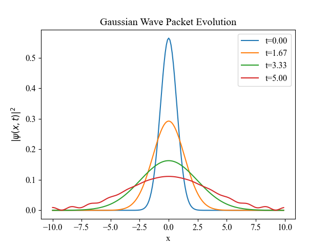
Figure 1. Evolution of a Gaussian wave packet over time, showing the probability density \( |ψ(x,t)∣^{2} \) at different time intervals. At \( (t=0.00 ) \) , the initial Gaussian wave packet. At \( (t_{1}=1.67) \) , the wave packet begins to spread. At \( (t_{2}=3.33) \) , the spread continues, showing increased uncertainty in position. At \( (t_{3}=5.00) \) , the wave packet is significantly dispersed.

3.2 Quantum Measurements:

Quantum measurement experiments frequently involve the precise determination of a particle's position or momentum [14], leading to inherent uncertainties described by the Heisenberg uncertainty principle. These uncertainties highlight the fundamental limits of measurement precision in quantum mechanics. In these experiments, the Fourier transform emerges as a powerful analytical tool, enabling researchers to analyze and interpret the resulting data more effectively. Consider a typical quantum measurement experiment that a particle with measured position [15]. The resulting wave function \( ψ(x) \) obtained from this measurement represents the probability amplitude of locating the particle at a specific position x. To gain insights into the momentum distribution of the particle, it is necessary to transform this wave function from the position space to the momentum space. This is achieved by applying the Fourier transform to \( ψ(x), \) resulting in \( ϕ(p), \) the wave function in momentum space. The wave function \( ϕ(p) \) provides a comprehensive understanding of the particle's momentum characteristics, complementing the positional information initially obtained.

\( ϕ(p)=\frac{1}{\sqrt[]{2πℏ}}\int_{R}^{} ψ(x)e^{-\frac{ipx}{ℏ}} dx\ \ \ (34) \)

By examining \( ϕ(p) \) , then can gain insights into the particle's momentum distribution.

The relationship between position and momentum uncertainties during a quantum measurement can be thoroughly analyzed using the Fourier transform. This mathematical technique allows people to convert the wave function from its original position representation to its momentum representation, providing a detailed insight into the distribution and interplay of these uncertainties. When measuring a particle's position with high precision, the wave function \( ψ(x) \) becomes sharply peaked, leading to a broad spread in \( ϕ(p) \) . This illustrates the trade-off between position and momentum uncertainties, as described by the Heisenberg uncertainty principle. To demonstrate this, consider experimental data where the position of a particle is measured multiple times. The resulting probability distribution \( P(x) \) can be Fourier transformed to obtain the momentum distribution \( P(p) \) . Using the experimental position data \( x_{i}, \) the author can construct the wave function:

\( ψ(x)=\sum_{i}^{} δ(x-x_{i})\ \ \ (35) \)

Applying the Fourier transform to \( ψ(x) \) , it is easy to get

\( ϕ(p)=\frac{1}{\sqrt[]{2πℏ}}\int_{R}^{} \sum_{i}^{} δ(x-x_{i})e^{-\frac{ipx}{ℏ}} dx=\frac{1}{\sqrt[]{2πℏ}}\sum_{i}^{} e^{-\frac{ipx_{i}}{ℏ}}\ \ \ (36) \)

By analyzing \( ϕ(p) \) , the author can visualize the momentum distribution corresponding to the measured positions.

To illustrate the application of the Fourier transform in analyzing quantum measurements, this paper can plot the frequency spectrum of the measurement results, see Figure 2. Consider an experiment where the position of a particle is measured, resulting in a set of position data points \( x_{i} \) . The Fourier transform of the position distribution \( P(x) \) gives the frequency spectrum \( P(p) \) . This spectrum reveals the contributions of different momentum components to the particle's wave function. Using the position data \( x_{i} \) from the experiment, the author can calculate the Fourier transform and plot the frequency spectrum. The plots show the position distribution \( P(x) \) and the corresponding momentum distribution \( P(p) \) obtained through the Fourier transform. This demonstrates how the Fourier transform can be used to analyze and interpret quantum measurement results, highlighting the relationship between position and momentum uncertainties.

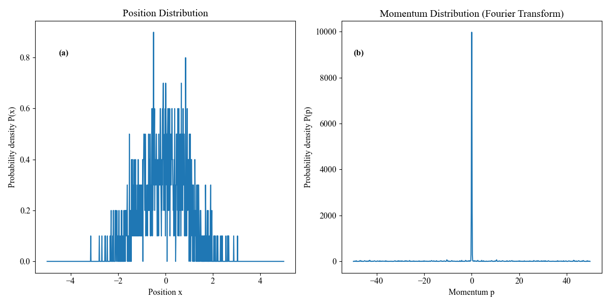
Figure 2. (a) Position distribution \( P(x) \) showing the probability density as a function of position \( x \) .(b) Momentum distribution \( P(p) \) obtained through Fourier transform, showing the probability density as a function of momentum \( p \) .

4 Conclusion

This paper systematically explores the significant applications and theoretical implications of the Fourier transform in quantum mechanics. By analyzing the Uncertainty Principle, the Planck-Einstein relation, and utilizing the Fourier transform to solve the Schrödinger equation, this paper demonstrates the extensive use of the Fourier transform as a fundamental tool in quantum mechanics. The Fourier transform provides a robust framework for understanding wave functions and their behavior in both position and momentum space at a theoretical level. Its application greatly simplifies the analysis and solution process of complex quantum systems in practice. Through specific case studies and numerical simulations, this paper showcases the practical applications of the Fourier transform in verifying the Heisenberg Uncertainty Principle and quantum measurements, further emphasizing its crucial role in quantum mechanic’s research. Additionally, the Fourier transform aids in illustrating the wave-particle duality and the probabilistic nature of quantum states, which are central to quantum theory. Looking ahead, with advancements in computational power and algorithm development, the integration of Fourier transform techniques with quantum computing and machine learning is expected to offer new possibilities for simulating and analyzing quantum systems with unprecedented precision. These developments could lead to breakthroughs into understanding and manipulation of quantum phenomena, reinforcing the indispensable role of the Fourier transform in the ongoing evolution of quantum mechanics.

References

[1]. Golse, F., & Paul, T. (2017). Empirical Measures and Quantum Mechanics: Applications to the Mean-Field Limit. Communications in Mathematical Physics, 369, 1021-1048.
[2]. Jaeger, G. (2015). Measurement and Fundamental Processes in Quantum Mechanics. Foundations of Physics, 45(2), 152-165.
[3]. Oppenheim, A. V., & Schafer, R. W. (1975). Digital Signal Processing. Prentice-Hall.
[4]. Kouba, O. (2013). A Mixed Parseval-Plancherel Formula. Journal of Classical Analysis, 4(1), 63-76.
[5]. Poojary, B. (2015). Origin of Heisenberg's Uncertainty Principle. American Journal of Modern Physics, 4(4), 193-198.
[6]. Gao, S. (2011). The Wave Function and Quantum Reality. Journal of Modern Physics, 2, 482-488.
[7]. Wang, X. (2009). The Cauchy-Schwarz Inequality and Its Applications. Mathematical Journal, 45(3), 203-217.
[8]. Williams, P. E. (2013). Phat photons and phat lasers. Proceedings of SPIE, 8841
[9]. Deng, X., & Deng, Z. (2022). The Matter Wave Is Space-Time Wave. Hypothesis and Theory Journal, 2(1), 60-75.
[10]. Livine, E. (2023). Evolution of the wave function's shape in a time-dependent harmonic potential. Europhysics Letters, 122(3), 1-12.
[11]. Ryan, F. (1988). Acoustic wave propagation employing Gaussian wave packets. The Journal of the Acoustical Society of America, 84(5), 1792-1799.
[12]. Li, H., Feng, B., & Wang, H. (2012). Gaussian Packets Modeling and Migration. The Journal of the Acoustical Society of America, 84(5), 1792-1799
[13]. Reimers, J., & Heller, E. (1985). The exact thermal rotational spectrum of a two-dimensional rigid rotor obtained using Gaussian wave packet dynamics. The Journal of Chemical Physics, 83(2), 516-523.
[14]. Wick, K. (2019). On the Quantum Mechanical Description of the Interaction between Particle and Detector. Physics, 3(4), 61.
[15]. Wan, K., & McLean, R. (1991). Are all quantum measurements reducible to local position measurements. Journal of Physics A: Mathematical and General, 24(8), 1681-1691.
Cite this article
Lyu,Y. (2024). Role of Fourier transform in quantum mechanics: Applications and implications. Theoretical and Natural Science,52,66-74.
Data availability
The datasets used and/or analyzed during the current study will be available from the authors upon reasonable request.
Disclaimer/Publisher's Note
The statements, opinions and data contained in all publications are solely those of the individual author(s) and contributor(s) and not of EWA Publishing and/or the editor(s). EWA Publishing and/or the editor(s) disclaim responsibility for any injury to people or property resulting from any ideas, methods, instructions or products referred to in the content.
About volume
Volume title: Proceedings of CONF-MPCS 2024 Workshop: Quantum Machine Learning: Bridging Quantum Physics and Computational Simulations
© 2024 by the author(s). Licensee EWA Publishing, Oxford, UK. This article is an open access article distributed under the terms and
conditions of the Creative Commons Attribution (CC BY) license. Authors who
publish this series agree to the following terms:
1. Authors retain copyright and grant the series right of first publication with the work simultaneously licensed under a Creative Commons
Attribution License that allows others to share the work with an acknowledgment of the work's authorship and initial publication in this
series.
2. Authors are able to enter into separate, additional contractual arrangements for the non-exclusive distribution of the series's published
version of the work (e.g., post it to an institutional repository or publish it in a book), with an acknowledgment of its initial
publication in this series.
3. Authors are permitted and encouraged to post their work online (e.g., in institutional repositories or on their website) prior to and
during the submission process, as it can lead to productive exchanges, as well as earlier and greater citation of published work (See
Open access policy for details).