1. Introduction

As an essential aspect of everyday life for the public, housing prices have consistently remained a matter of great importance. From 2004 onward, there has been a sustained nationwide escalation in housing prices in China, making it a central point of interest in the daily lives of individuals [1]. In China, mean house prices almost doubled from 2002 to 2010, indicating substantial fluctuations in house prices over the span of a few years [2]. The fluctuation in housing market prices has affected the daily consumption patterns of both urban and rural dwellers in China [3]. Also, housing price fluctuations significantly inhibit total factor productivity, which hindered economic development [4]. The similar thing happened in America. In the 80s and early 90s of the 20th century, housing prices in the United States maintained a steady upward trend, but Boston’s housing prices fluctuated significantly, Boston’s housing prices began to rise rapidly in 1983, and Boston’s housing prices began to turn around in the third quarter of 1988, and it took four full years to get out of the shadow of the decline, which has had a certain impact on the economic development of Boston area [5]. Hence, housing prices fluctuations not only affect life of residents worldwide, but also hindered economic development in a certain degree. It shows that it is important to get an accurate housing prices prediction model to assist people in assessing the planned purchase of a house and government regulate housing prices for better economic development.

Many house prices prediction works have been carried out. Chen and Qing analyzed the influencing factors of housing prices in different communities in the Boston area in 1980, using quantile regression as the basic method, and preliminarily explores the factors that affect the high or low prices of houses in different areas or communities in a region, besides the level of economic development. The use of quantile regression avoids the strict limitations of traditional ordinary least square (OLS) methods on data distribution characteristics and enables targeted research on different data at different quantiles [6]. Wang used the Boston housing price data, this study compares four methods: Levenberg-Marquardt, robust linear regression, Least Mean Squares, and tau. The focus is on analyzing the classic estimation methods and three robust estimation methods, studying the differences and advantages and disadvantages of the four methods [7]. But there exists a shortage of precision. Tian utilized a range of techniques to address the practical issue of predicting house prices in Boston, employing diverse methods for training and testing. It conducted a comprehensive comparison of diverse algorithm models, evaluating their performance from various perspectives and drawing conclusions about their effectiveness. It conducted a horizontal comparison of the advantages and weaknesses of various models and analyzed and summarized the differences in effectiveness [8]. Li and Guo considered the statistical diagnosis and local influence analysis of the single index mode based on data deletion and mode drift models. Simulation studies and results demonstrate the effectiveness and feasibility of the proposed method [9]. This article uses the typical and authoritative Boston housing price data as an example of the application of the semi-parametric varying coefficient quantile regression model and its two-stage estimation, demonstrating the model's good explanatory power in real economic issues [10].

In conclusion, this research compared different algorithmic models from multiple perspectives in order to provide an analysis and summary of their performance in predicting Boston house prices as a regression problem.

2. Methodology

2.1. Data source and description

The data utilized in this paper was sourced from the StatLib library, which is curated at Carnegie Mellon University. It contains 13 continuous attributes, 1 binary-valued attribute and 506 rows.

2.2. Variable selection

The Boston housing price data is relatively clean, so the preprocessing and feature engineering work will be relatively minimal. There are no missing values in the datasets. And the datasets don't contain attributes with low correlation, and there's no need to worry about multicollinearity. Eventually, all features are included. The data that the current paper analyzed contains 13 independent variables and one dependent variable (PRICE). The detailed information of this datasets is displayed in Table 1.

Table 1. Features interpretation.

2.3. Method introduction

The paper compares four different methods: Multiple Linear Regression, Random Forest Regression, Extreme Gradient Boosting Regression, Support Vector Machine Regression. After analyzing the advantages and disadvantages of the four methods, the most suitable model was selected to construct a Boston housing prices prediction model based on the datasets.

In machine learning, Multiple Linear Regression is a statistical technique employed to forecast the linear correlation between several independent variables and a dependent variable. Within this method, the association is represented as a linear equation, in which the dependent variable is a weighted total of the independent variables, coupled with an intercept term. Random Forest Regression functions by creating numerous decision trees during the training process and produces the average prediction from each tree for regression assignments. Every tree is constructed using a random subset of the training data and a random subset of the features, aiding in diminishing overfitting and enhancing overall applicability. Extreme Gradient Boosting Regression operates by constructing a sequence of decision trees, with each subsequent tree rectifying the errors of its predecessor. A technique named gradient boosting is used to minimize the loss function by adding new models to the ensemble in a step-by-step fashion. Support Vector Machine regression aims to determine the optimal hyperplane that effectively segregates data points belonging to distinct classes within a high-dimensional space. It is applicable for both classification and regression assignments.

3. Results and discussion

3.1. Multiple linear regression

The mathematical formula for multiple linear regression is:

\( E(Y)={β_{0}}+{β_{1}}{x_{1}}+{β_{2}}{x_{2}}+⋯+{β_{13}}{x_{13}}+e\ \ \ (1) \)

In the above formula: \( {β_{0}} \) is a constant term, and e is a residual term.

According to the heatmap, the independent variables do not exhibit highly correlated features among themselves and there are no features with relatively low correlation with the target variable (Figure 1). There is also no need to worry about multicollinearity.

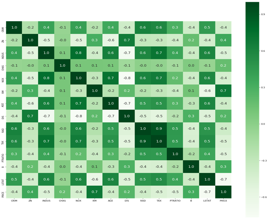
Figure 1. Heatmap of correlation between features.

Table 2. Model results.

Regression outcomes are shown in the above (Table 2). The significance for the 11 independent variables did not exceed 0.002, which indicates that each of 11 independent variables has a notable influence on the dependent variable Y. To evaluate the model, visualization figure of actual prices compared to predicted prices is shown below (Figure 2).

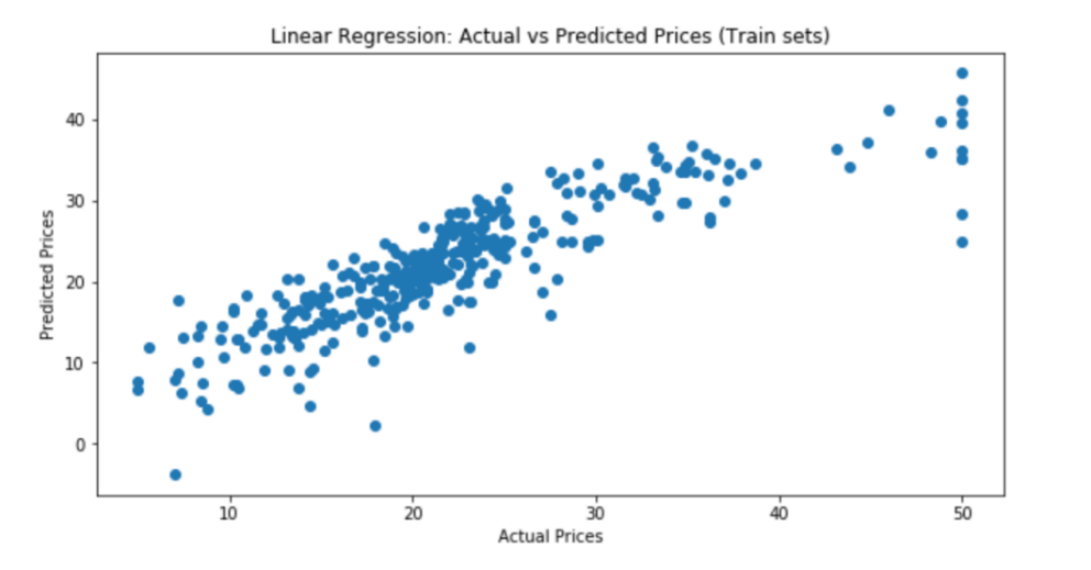
Figure 2. Actual prices compared to predicted prices (multiple linear regression).

The visualized graph indicates that this is not a very good model in terms of intuitive effect. The deviation between predicted values and actual values is not slight enough to be ignored, which indicates that the model's fitting effect is not good (Table 3).

Table 3. Model Evaluation (Multiple Linear Regression).

In order to evaluate the model and compare with other three models later more accurately, five data are shown in figure 3. R-squared score is 0.712. Adjusted R-squared score is 0.685. Mean absolute error is 3.867. Mean squared error is 30.068. Root mean squared error is 5.483.

3.2. Random forest regression

Random Forest Regression is renowned for its robustness, flexibility, and capacity to manage high-dimensional extensive datasets, making it a popular choice for predictive modeling in various domains.

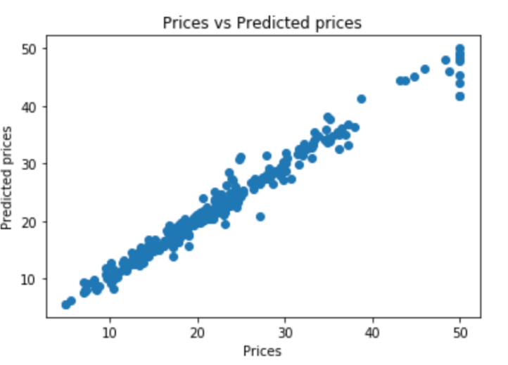
Figure 3. Actual prices compared to predicted prices (random forest regression).

Figure 3 compares actual prices and predicted prices in the training set. If fitting all the points in the figure 3, the line is close to the line y=x. It turns out that the model has good generalization ability by visualization.

Table 4. Model evaluation (random forest regression).

R-squared for Random Forest Regression is 0.822. Adjusted R-squared is 0.805. Mean absolute error is 2.469. Mean squared error is 18.619. Root mean squared error is 4.315 (Table 4).

3.3. Extreme gradient boosting regression

Extreme Gradient Boosting Regression is renowned for its high performance, flexibility, and excellent predictive capabilities, making it an essential tool for addressing regression problems.

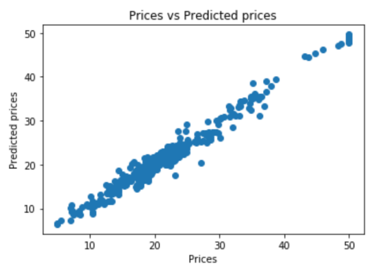
Figure 4. Actual prices compared to predicted prices (XGBoost regression).

By visualization, it is evident that the Extreme Gradient Boosting model exhibits good fitting and generalization capabilities, notably outperforming the multiple linear regression model (Figure 4).

Table 5. Model Evaluation (Extreme Gradient Boosting Regression).

For Extreme Gradient Boosting Regression model, R-squared is 0.849. Adjusted R-squared is 0.835. Mean absolute error is 2.451. Mean squared error is 15.716. Root mean squared error is 3.964 (Table 5).

3.4. Support vector machine

Benefits of Support Vector Machine Regression include efficacy with high-dimensional domains, robustness to overfitting, versatility in kernel selection, and suitability for non-linear data.

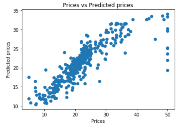
Figure 5. Actual prices compared to predicted prices (SVM egression).

Figure 5 shows the comparison of actual prices with prices predicted by Support Vector Machine Regression model. The scattered distribution of points in the graph indicates that the model has poor fitting and generalization capabilities.

Table 6. Model Evaluation (Support Vector Machine Regression).

In fact, five evaluation index shown in table 6 reflects poor fitting and generalization capability of Support Vector Machine Regression model. R-squared is as low as 0.590. Adjusted R-squared is 0.551. Mean absolute error is 3.756. Mean squared error is as large as 42.811. Root mean squared error is 6.543.

3.5. Comparison of four models

In summary, table 7 gives a direct comparison of four regression models. Upon analyzing the performance of the four models, it is evident that Extreme Gradient Boosting Regression model demonstrates the highest R-squared and adjusted R-squared values, the lowest mean absolute error, mean squared error and root mean squared error. Therefore, Extreme Gradient Boosting Regression appears to be the most effective model among the four models.

Table 7. Comparison Table for Four Models.

4. Conclusion

The study applied four different regression methods to the datasets derived from the StatLib library. Upon analyzing R-squared value, adjusted R-squared value, mean absolute error, mean squared error and root mean squared error, Extreme Gradient Boosting Regression was found to be the most effective model to predict Boston housing prices.

By the Boston housing prices prediction model using Extreme Gradient Boosting regression, the government can use the predictive results of the Boston housing price prediction model to formulate real estate policies such as rational planning of housing construction and controlling housing prices to promote sustainable urban development. For the general public and investors, the Boston housing price model can provide them with references when purchasing houses, helping them make wiser home purchasing and investment decisions. However, there are also some drawbacks. The model is based on historical data for prediction, and may not accurately predict the impact of future economic changes, policy adjustments, and other factors. And predictive results of the model are typically aimed at overall trends and may have errors in assessing the specific value of individual properties, unable to fully cover individual differences.

References

[1]. Wu Z K, Tang W G and Wu B 2007 Using the Priority Factor Method to Analyze the Impact of House Price Factors on Buyers' Orientation. Journal of Tianjin University of Commerce, 27(3).
[2]. Hu Q 2017 Analysis of housing price factors based on the SVAR model. Times Finance.
[3]. Yang D X and Zhang Z M 2013 An empirical study on incorporating housing price factors into China's CPI. Statistics&Information Forum, 28(3).
[4]. Li J, Chen Y and Guo W 2024 Will housing price fluctuations suppress total factor productivity growth? Empirical analysis based on 259 prefecture-level and above cities in China. Hainan Finance, 5, 3-21.
[5]. Yu X F 2002 Potential risks facing the current residential housing industry in Zhejiang from the perspective of international experience: Lessons from the substantial fluctuations in housing prices in Los Angeles and Boston from 1983 to 1993. Journal of Zhejiang University of Technology, 3.
[6]. Chen Z and Qing Q 2015 Factors affecting housing prices in different communities in Boston: Based on quantile regression analysis. Business, 30, 278-279.
[7]. Wang Y 2019 A review of research on Boston housing prices based on classical and robust methods. Market Weekly, 3, 40-43.
[8]. Tian R 2019 Boston housing price prediction based on multiple machine learning algorithms. China New Communication, 11, 228-230.
[9]. Li H, Zhu G and Guo Z 2017 Statistical diagnosis of single index mode and its application in the analysis of Boston housing prices. Statistical Research and Management, 6, 1091-1105.
[10]. Weng Y 2009 Semi-parametric varying coefficient quantile regression model and its two-stage estimation, Doctoral dissertation, Xiamen University.
Cite this article
Liu,B. (2024). Research on housing prices prediction-take Boston as an example. Theoretical and Natural Science,52,171-178.
Data availability
The datasets used and/or analyzed during the current study will be available from the authors upon reasonable request.
Disclaimer/Publisher's Note
The statements, opinions and data contained in all publications are solely those of the individual author(s) and contributor(s) and not of EWA Publishing and/or the editor(s). EWA Publishing and/or the editor(s) disclaim responsibility for any injury to people or property resulting from any ideas, methods, instructions or products referred to in the content.
About volume
Volume title: Proceedings of CONF-MPCS 2024 Workshop: Quantum Machine Learning: Bridging Quantum Physics and Computational Simulations
© 2024 by the author(s). Licensee EWA Publishing, Oxford, UK. This article is an open access article distributed under the terms and
conditions of the Creative Commons Attribution (CC BY) license. Authors who
publish this series agree to the following terms:
1. Authors retain copyright and grant the series right of first publication with the work simultaneously licensed under a Creative Commons
Attribution License that allows others to share the work with an acknowledgment of the work's authorship and initial publication in this
series.
2. Authors are able to enter into separate, additional contractual arrangements for the non-exclusive distribution of the series's published
version of the work (e.g., post it to an institutional repository or publish it in a book), with an acknowledgment of its initial
publication in this series.
3. Authors are permitted and encouraged to post their work online (e.g., in institutional repositories or on their website) prior to and
during the submission process, as it can lead to productive exchanges, as well as earlier and greater citation of published work (See
Open access policy for details).