1. Introduction

The Support Vector Machine (SVM) is the cornerstone of the machine learning field. They have high efficiency when solving classification and regression tasks. The classical SVM uses mathematical concepts such as margins and support vectors to classify data points by finding the best hyperplane.

However, as the amount of data increases, it becomes very complex. The shortcomings of the classical SVM become more and more obvious, especially when it solves high-dimensional data tasks and the computational speed decreases a lot. The quantum computing solves these challenges. Quantum Support Vector Machines (QSVMs) utilize the properties of quantum mechanics, such as superposition and entanglement, to provide a brand new method for machine learning.

This paper explores the combination of quantum computing principles and classical SVMs to enhance machine learning performance. This paper explain the fundamental concepts of classical SVMs, including hyperplanes, margins, support vectors, and kernel methods. Then deeply explain the fundamental concepts of quantum computing, such as quantum bits, quantum states, and quantum gates, etc.

One of the main topics of the paper is the theoretical advantages of QSVM, including faster computation speeds and higher performance with handle high-dimensional data. The research highlights how QSVMs utilize quantum algorithms and kernel methods to compute complex kernel functions that are difficult for classical computers to handle. Quantum algorithms provide new computational methods that can speed up many kinds of machine learning tasks. In addition, the paper discusses practical considerations for implement of QSVMs, such as quantum hardware requirements and error mitigation techniques, which are essential for real-world applications of QSVMs.

This paper illustrates the potential of quantum support vector machines to utilize quantum computing to advance machine learning. QSVMs provides a more accurate and faster way to compute.

2. Fundamentals of Support Vector Machine (SVM)

To solve problems of classification and regression, the author use Support vector machine (SVM) . It has good robustness in high dimensional spaces and have high efficiency in image recognition.

2.1. Basic Concepts: Hyperplanes, Margins, and Support Vectors

Hyperplane is the most important concept of SVM, which is a decision boundary. As shown in Figure 1, it was used to separate different categories in the feature space. For two different categories of datasets, the author needs to find the hyperplane firstly. The distance between nearest data points(support vectors) and the hyperplane for each type of data is called margin, the author needs to maximize it.

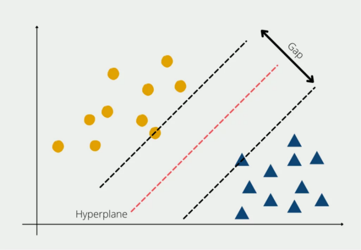
Figure 1. The horizontal and vertical axes depend on the units of our data. The red dash line represent hyperplane in 2D. The navy blue triangles and yellow circles represent two different data categories. The gap between two black dash line represent margin. The data points crossed by the black dash line are called support vectors.

2.2. Training and Optimization

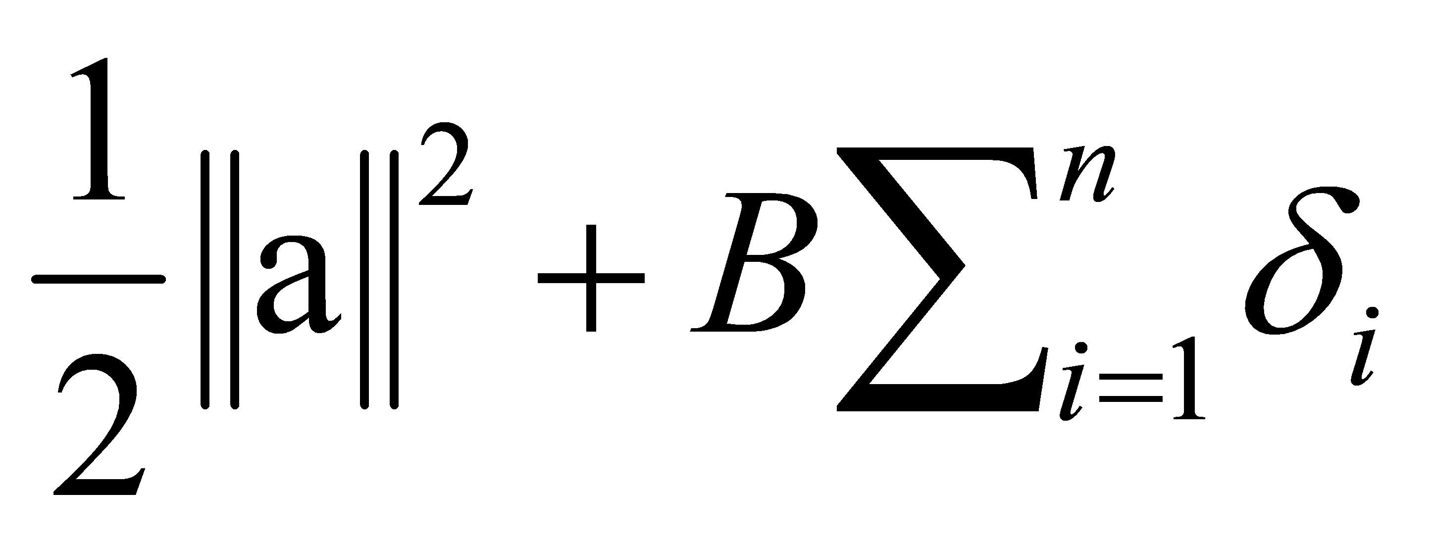
Training an SVM requires solving a quadratic optimization problem with linear constraints. This process is computationally intensive, especially for large datasets. The author needs to minimize it[1]:

(1)

(2)

where a is called weight vector, c is called bias term, 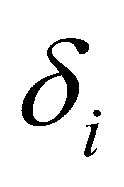are called slack variables and 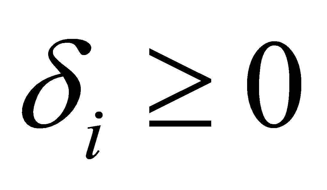, B is called regularization parameter that keep balance between the margin(maximize) and the classification error(minimize), \( {x_{i}} \) are the training examples. And \( {y_{i}} \) are the corresponding labels, usually equal to 1 or -1, depending on the category of data points.

2.3. Kernel Methods

The kernel method for nonlinear classification is one of the most powerful features of SVM . Mapping the data that we input into a higher dimensional space is called kernel, it is a function. In addition, it does not need to get the coordinates of data. In the transformed feature space, kernel methods allows SVM can find a linearly separating hyperplane. In original input space, it corresponds to the non-linear boundary.

Here are some Commonly kernels[2]:

Linear Kernel: (3)

It is suitable when the data seem to be linearly separable and when there is a low risk of overfitting.

It usually does not require too much computational performance.

Polynomial Kernel: (4)

where c is constant.

It is suitable when the data have nonlinear relationships. It is also easier to interpret than some other nonlinear kernels like the RBF kernel. Compared to linear kernels, polynomial kernel require more computational performance.

In addition, there are many other kernels, such as the Radial Basis Function Kernel, Gaussian Kernel, Sigmoid Kernel, Laplacian Kernel, etc.

Each kernel function provides a different way to measure similarity between data points, it allows the SVM to capture relationships between data category.

SVM’s performance depends on kernel method that the author choose, the regularization parameter, other hyper-parameters, etc. Proper validation are essential to achieving optimal results. Properly adjusted parameters also produce better results.

In summary, classical SVMs are powerful tools in machine learning. They provide a framework for understanding more advanced concepts such as Quantum Support Vector Machines, which use quantum computing to increase the performance of SVMs.

3. Quantum Computing Basics

The quantum computing represents an evolution in computing technology. It utilizes quantum mechanics to process data in a new way.

3.1. Qubits and Quantum States

The essential concept of quantum information is the quantum bit. Classical bit can only represent 0 or 1, but qubits can represent a superposition of two states meanwhile. This property is derived from the principles of quantum mechanics, it allows a quantum bit to perform multiple computations at the same time. The author uses Hilbert space to represent the state a vector(qubit), usually written as , where and are complex coefficients, and it satisfies [3].

3.2. Quantum Superposition and Entanglement

Superposition allows combined states of and to represent a qubit. The combination of states allows for parallelism in quantum computing. Another critical phenomenon is entanglement, where the quantum states have two or more quantum bits, and they are interdependent. Entangled quantum bits have stronger correlations than any other classical system. It means the state of one quantum bit will be affected by the state of other quantum bit immediately, in spite of how far between them. It is important for most quantum algorithms. It provides the basis for quantum communication and computation[4].

3.3. Bloch sphere

The author uses bloch sphere which is a suitable way to represent the state of a quantum bit. It is a visual model of a qubit’s quantum state. As shown in Figure 2, a unit sphere in three-dimensional space, any points in the sphere can represent one possible state of a quantum bit.

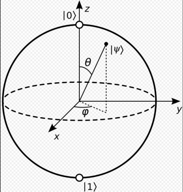
Figure 2. on positive z axis represent the classical bit value 0. on negative z axis represent the classical bit value 1. Equator represents superpositions ofandwith equal probabilities but different relative phases.

In the Bloch sphere representation, this state is expressed using two real parameters: the azimuthal angle \( φ \) and the polar angle θ[5]:

(5)

3.4. Quantum Gates and Circuits

The quantum gate is the fundamental element in quantum circuits, similar to classical logic gates in digital circuits. As shown in Table 1, these gates operate the quantum bits through unitary transformations, they change their state according to specific quantum rules.

Table 1. This table lists some Pauli gate and some other quantum gates[6].

A series of quantum gates constitute quantum circuit that allow quantum bits to perform computational tasks. Quantum circuits are similar to classical circuits. Qubits are usually initialized to a specific state, usually . Then Quantum gates are applied to the qubits in a specific sequence.

For instance, applying a Hadamard gate, and then applying a CNOT gate can create an entangled state. After the gates have been applied, the qubits are measured. Measurement can cause the collapse of the qubits from their quantum superpositions to classical states. It provided the final output of the computation.

A Bell state is a specific type of entangled state. There are four Bell states. Here the author discusses the most common one[7]:

(6)

This circuit involves two main quantum gates: the Hadamard gate and the Controlled-NOT gate.

Start with two qubits in the initial state (Define). Then apply the Hadamard Gate to Qubit 1, the Hadamard gate transfers the first qubit into a superposition state:

(7)

After applying the Hadamard gate, the state is:

(8)

Then apply the CNOT Gate:

(9)

3.5. Quantum Algorithms Relevant to Machine Learning

Quantum Approximate Optimization Algorithm (QAOA) can find approximate solutions to optimization problems more efficiently than traditional algorithms. It does well in scheduling, resource allocation, and machine learning model optimization. QAOA starts with a superposition of all possible solutions. Then, it uses a sequence of quantum gates that encode the problem constraints and the objective function. Finally, it optimizes the parameters to maximize the probability of measuring the optimal solution[8].

Traditional PCA algorithms are difficult to handle when dealing with large data, but QPCA may have much faster speed. It encodes the the data’s covariance matrix into a quantum state. Then, it uses it to estimate the eigenvalues and the eigenvectors of the covariance matrix. Finally, it measures the quantum state to extract the principal components.

Quantum Support Vector Machine (QSVM) can more efficiently handle high-dimensional data and large datasets than classical SVM, it provides faster speed and accuracy. QSVM uses quantum circuits to compute the kernel matrix, which measures the similarity in a higher-dimensional space. Then use quantum algorithms to address the quadratic optimization problem. Finally, use the trained quantum model to classify new data points.

There are many other kinds of quantum algorithms for machine learning, the author does not list all quantum algorithms.

4. Quantum Support Vector Machines (QSVMs)

The QSVM enhance classical SVM by using quantum computing principles to process high-dimensional data more efficiently. Including encoding data into quantum states, and measuring the quantum states. By utilizing superposition and entanglement, QSVMs can significantly improve computational efficiency and accuracy. The conceptual framework of QSVM consists of the following components:

4.1. Quantum Data Encoding

Amplitude Encoding uses the amplitudes of a quantum state to represent data. For example, a data vector , can be encoded into a quantum state , where are the basis states[9]. Basis Encoding uses the basis states of the qubits to represent traditional binary data. For example, a binary string 1101 can be encoded directly into the state [10]. Angle Encoding is make data encoded into the rotation angles of qubits. This is often used in combination with other encoding methods to represent more complex data.

4.2. Quantum Kernel Methods

Quantum kernel methods extend classical kernel methods, by utilizing quantum states and quantum circuits to compute the kernel function. The quantum kernel function is defined as the inner product of quantum states:

(10)

where the inner product measures the similarity between the quantum states, it is similar to classical kernel functions[11].

4.3. Implementing SVMs on Quantum Computers

To encode classical data into quantum states, the author uses methods such as basis encoding or amplitude encoding. Designing quantum circuits to prepare these states. Quantum circuits compute the kernel matrix, which gets the similarity between input data points. Variational Quantum Eigensolver (VQE) or Quantum Approximate Optimization Algorithm (QAOA), are used to solve the optimization problem. The trained quantum SVM model can classify new data points by evaluating them in the quantum feature space[11].

On quantum computers, training SVM use quantum algorithms to optimize the model parameters. Here are some important quantum algorithms: Harrow-Hassidim-Lloyd (HHL) Algorithm, Quantum Support Vector Classification (QSVC), Quantum Principal Component Analysis (QPCA)

4.4. Quantum Gradient Descent

In QGD, the parameters of the quantum machine learning model are often represented as quantum states. Quantum circuits are used to compute gradients. Usually use parameter-shift rule to compute[12]:

If is a parameterized quantum gate and is the expectation value of an observable O, the gradient of can be estimated as:

(11)

After computing the gradient, the parameters of the quantum model are updated:

(12)

where is called learning rate.

Computing the quantum gradient and updating the parameters is iteratively repeated. The algorithm will continue until it attains the stopping criteria. In QSVM, QGD is used to optimize the parameters of the quantum kernel and maximizes the margin(decision boundary) between classes in the transformed feature space.

4.5. Quantum Measurement and Output Interpretation

Once the quantum circuit has completed its computations, the final step is to measure the quantum state to get the results. Measurement collapses the quantum state into classical information, which can be predicted or categorized by interpreting the classical information. Each measurement outcome has probabilities, which depend on probability amplitude of the quantum state. Classical post-processing may be required to interpret the measurement results, and the author needs to use them for decision-making in the SVM model.

5. Theoretical Advantages of QSVMs

The Quantum Support Vector Machine have a series of theoretical advantages over Classical Support Vector Machines, mainly due to the properties of quantum computing. These advantages can improve the performance of machine learning models, especially when solve with more complex and higher dimensional data. The author will discuss the theoretical advantages of QSVMs: computational speedup, handling of high-dimensional data, and improved kernel computation.

5.1. Computational Speedup

5.1.1. Quantum Parallelism

It allows a quantum computer to process multiple inputs simultaneously according to the superposition principle, . In classical computing, classical bit can only represent two states (either 0 or 1). But a quantum bit can represent a superposition of two states.

5.1.2. Simultaneous Computation

When multiple quantum bits are entangled, a quantum computer can compute a huge number of states simultaneously. If a system has n qubits, the largest number of states is 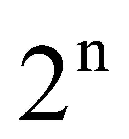. This parallelism allows quantum computers to compute many possible solutions at the same time.

5.2. Handling High-Dimensional Data

Quantum computing has unique advantages to solve these challenges. With the number of quantum bits increases, the quantum state space exponential increases. Quantum computers can easily operate in very high-dimensional spaces. This allows QSVM to process high-dimensional data more efficiently. Quantum kernel methods can compute the inner products of quantum states more efficiently than classical methods. These inner products form the kernel matrix, which is essential for SVM training. Quantum circuits can evaluate complex kernel functions that are infeasible for classical computers. Quantum circuits can compute complex kernel functions that classical computers can not do.

6. Implementation of QSVMs

6.1. Quantum Hardware Requirements and Practical Considerations

QSVMs require a sufficient number of qubits to represent the data. It depends on the size and complexity of the dataset. For example, if a dataset has n features, then it may require 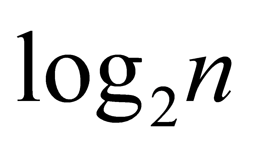qubits for basic encoding. Connectivity between qubits is important for implementing complex quantum circuits. Long coherence times are necessary to maintain quantum states during computation. However, longer coherence times will reduce the likelihood of decoherence. It will produce errors during the computation. At high temperatures, thermal noise in the environment influences the stability of quantum bits and leads to computational errors. By cooling the quantum computer to extremely low temperatures, the background thermal noise can be reduced. But cooling to extremely low temperatures is also a challenge. QSVM algorithms often require deep quantum circuits. The number of sequential quantum gates is called depth. However, more quantum gates are more likely to produce errors.

6.2. Error Mitigation

Error mitigation is an important technique of quantum computing, especially for implementing Quantum Support Vector Machines. Due to the nature of quantum states and the current limitations of quantum hardware, various techniques are used to reduce the impact of errors, such as Quantum Error Mitigation Techniques, Quantum Error Correction Codes, Noise-Aware Compilation, etc.

In Zero-Noise Extrapolation, it runs the quantum circuit at different artificial noise levels and extrapolates the results back to the zero-noise case. By adding noise and measuring the results, the author can extrapolate what the results would have been if there was no noise. Surface code is a topological code that arranges quantum bits in a two-dimensional lattice. It can correct errors by measuring special information from surrounding quantum bits. When designing quantum circuits, it is important to make them more resistant to noise. This includes minimizing circuit depth and optimizing gate sequences to reduce the overall probability of error[13].

Error reduction is important for the practical implementation of QSVM on current quantum hardware. Error mitigation techniques provide ways to reduce errors without expending too much resources. By using a combination of these techniques, the reliability and accuracy of QSVM can be increased.

7. Conclusion

This paper explores the integration of quantum computing principles with classical support vector machines (SVMs) to improve machine learning performance. It begins with the classical SVMs, emphasizing their efficiency in classification and regression tasks, but highlighting their limitations in handling high-dimensional data and computational speed.

Quantum computing uses qubits, superposition, and quantum entanglement to enable parallelism and faster computation. It also solves the limitations of classical SVMs. The paper deeply discusses the components of Quantum Support Vector Machines (QSVMs), such as quantum data encoding, quantum kernel methods, and the implementation of SVMs on quantum computers. QSVMs utilize quantum circuits to compute kernel matrices more efficiently which has advantages in processing complex and high-dimensional data.

The paper emphasizes the theoretical advantages of QSVMs over classical SVMs, including faster computation and better kernel computation through quantum parallelism. The paper also explores the practical challenges of implementing QSVMs, such as quantum hardware requirements, error mitigation techniques, and the requirement for deep quantum circuits.

In conclusion, this paper shows that quantum support vector machines solve the computational limitations of classical SVMs. The combination of quantum computing and SVM principles can handle large and complex datasets more efficiently, which can improve the speed and accuracy of machine learning applications. However, to fully utilize the performance of QSVM, we need to solve the problems in practical applications, especially those related to quantum hardware.

References

[1]. Jakkula V. Tutorial on support vector machine (svm)[J]. School of EECS, Washington State University, 2006, 37(2.5): 3.
[2]. Campbell C. An introduction to kernel methods[J]. Studies in Fuzziness and Soft Computing, 2001, 66: 155-192.
[3]. Williams C P. Explorations in quantum computing[M], pages 9-21, Springer Science & Business Media, 2010.
[4]. McIntyre D H. Quantum mechanics[M], pages 97-106, Cambridge University Press, 2022.
[5]. Glendinning I. The bloch sphere[C]//QIA Meeting. 2005: 3-18.
[6]. Williams C P, Williams C P. Quantum gates[J]. Explorations in Quantum Computing, 2011: 51-122.
[7]. Weigold M, Barzen J, Leymann F, et al. Encoding patterns for quantum algorithms[J]. IET Quantum Communication, 2021, 2(4): 141-152.
[8]. Cerezo M, Arrasmith A, Babbush R, et al. Variational quantum algorithms[J]. Nature Reviews Physics, 2021, 3(9): 625-644.
[9]. Weigold M, Barzen J, Leymann F, et al. Encoding patterns for quantum algorithms[J]. IET Quantum Communication, 2021, 2(4): 141-152.
[10]. Schuld M, Killoran N. Quantum machine learning in feature hilbert spaces[J]. Physical review letters, 2019, 122(4): 040504.
[11]. Singh G, Kaur M, Singh M, et al. Implementation of quantum support vector machine algorithm using a benchmarking dataset[J]. Indian Journal of Pure & Applied Physics (IJPAP), 2022, 60(5).
[12]. Anwar M S. A Review of Quantum Gradient Descent[J].
[13]. Cai Z, Babbush R, Benjamin S C, et al. Quantum error mitigation[J]. Reviews of Modern Physics, 2023, 95(4): 045005.
Cite this article
Yin,T. (2024). Quantum support vector machines: theory and applications. Theoretical and Natural Science,51,34-42.
Data availability
The datasets used and/or analyzed during the current study will be available from the authors upon reasonable request.
Disclaimer/Publisher's Note
The statements, opinions and data contained in all publications are solely those of the individual author(s) and contributor(s) and not of EWA Publishing and/or the editor(s). EWA Publishing and/or the editor(s) disclaim responsibility for any injury to people or property resulting from any ideas, methods, instructions or products referred to in the content.
About volume
Volume title: Proceedings of CONF-MPCS 2024 Workshop: Quantum Machine Learning: Bridging Quantum Physics and Computational Simulations
© 2024 by the author(s). Licensee EWA Publishing, Oxford, UK. This article is an open access article distributed under the terms and
conditions of the Creative Commons Attribution (CC BY) license. Authors who
publish this series agree to the following terms:
1. Authors retain copyright and grant the series right of first publication with the work simultaneously licensed under a Creative Commons
Attribution License that allows others to share the work with an acknowledgment of the work's authorship and initial publication in this
series.
2. Authors are able to enter into separate, additional contractual arrangements for the non-exclusive distribution of the series's published
version of the work (e.g., post it to an institutional repository or publish it in a book), with an acknowledgment of its initial
publication in this series.
3. Authors are permitted and encouraged to post their work online (e.g., in institutional repositories or on their website) prior to and
during the submission process, as it can lead to productive exchanges, as well as earlier and greater citation of published work (See
Open access policy for details).