1. Introduction

Medical insurance is an important form of risk management in people’s life. In case of major diseases, it helps people to get through these difficulties by paying for their treatments and medical expenses. However, the cost of medical insurances can be exceptionally high as it varies from one insurer to another. People with bad habits or unhealthy life style are more likely to be charged a higher insurance price because they are prone to major diseases. This paper uses a medical insurance dataset from Kaggle to study the potential cause of high insurance charges. Since this dataset contains not only charges but also other important information of the insurer, it is suitable to implement exploratory analysis on this dataset and discover the statistical relationship between insurers’ characteristics and their insurance charges.

In the dataset, each row represents an individual insurer. In a single row, the first six columns represent characteristics about the insurer, and the last column is the medical insurance charge that person needs to pay for. These characteristics all contribute to the final pricing of the insurance, but they do not contribute equally.

It is expected that smoking and high body mass index (bmi) contribute more to higher charged, which will be discussed in the result section [1]. The author also constructed a multilinear regression model to predict the insurance charges. The multiple linear regression (MLR) equation is expected be \( {h_{θ}}({x_{i}})={θ_{0}}+{θ_{1}}{x_{i1}}+{θ_{2}}{x_{i2}}+…+{θ_{n}}{x_{mn}} \) where θ is the parameter of each characteristic of the insurers, x is the dependent variable like age and bmi, n is the number of variables, and m is the number of trails. For this dataset, the multilinear regression equation is \( {h_{θ}}({x_{i}})={θ_{0}}+{θ_{1}}age+{θ_{2}}sex+{θ_{3}}bmi+{θ_{4}}children+{θ_{5}}smoker+{θ_{6}}region \) . For example, the MLR formula for the first insurer will be written like this: \( 16884.92400={θ_{0}}+{θ_{1}}*19+{θ_{2}}*female+{θ_{3}}*27.900+{θ_{4}}*0+{θ_{5}}*smoker(yes)+{θ_{6}}*southwest \) . The author uses Python to construct this MLR model and test its accuracy.

2. Literature review

Tranmer et al. explained multilinear regression as an extension of simple linear regression [2]. It is a statical model that can be applied to predict one dependent variable Y from a collection of independent variables ( \( {x_{1}}→{x_{n}} \) ). The dataset presented in this paper is suitable for multilinear regression because the dependent variable charge is determined by several independent variables like age and sex.

Although this statistical model is advantageous in forecasting outcomes from various variables, there can be drawbacks associated with it. In case where the relationship between different variables is complex, it is difficult to examine which variables will possibly pollute the linear relationship due to multicollinearity [3].

A good example of implementing MLR is found in the work of Uyanık et al. [4]. They constructed an MLR model on State Employees Selection Exam (KPSS) scores. They use five other scores like course evaluation scores and guidance scores as their independent variables to predict the dependent variable: KPSS score. Their MLR model achieve a successful R-Squared score of 0.87 which indicates that MLR should be effective on similar dataset like the one in this paper. Moreover, using MLR allows all possible variables that can affect the final outcome to be considered.

Similarly, Rossi et al. tried to predict the specific methane production (SMP) using several other chemicals [5]. They first develop a simple linear regression model using only the most correlated chemical, lignin, to predict the SMP. The resulting model is unsatisfactory with a low R-Squared score of 0.3. Consequently, they develop a MLR model including all variables correlated to the SMP, which results in a successful model with a high R-Squared score of 0.87. Moreover, Rath et al. collected COVID-19 data from World Health Organization to predict the number of active cases next day [6]. Their MLR model produce a high R-Squared score which shows the potential of using MLR in predicting the spread of contagious diseases.

The size of sample size is also an important factor in producing a successful MLR model [7]. As Knofczynski et al. showed in their work, the Squared Population Multiple Correlation decreases as the sample size increases. It is important to increases sample sizes if dataset has a large number of independent variables.

One drawback of MLR model is that the common measurements like mean square error and R-Squared only test the goodness of fit of the model but not the accuracy of the prediction [8, 9]. In some circumstances where the performance of the model is need, other methods like Random Forest may need to be applied [10].

3. Methodology

3.1. Data source

The data for this paper is retrieved from Kaggle. The original data is from Brett Lantz’s Machine Learning with R, and it is available on GitHub. Miri Choi reposted this dataset from GitHub to Kaggle.

3.2. Variable selection

Table 1 below shows the first five rows of the dataset. The dataset contains 1336 insurers with 51% male and 49% female. The dataset contains 7 variables: the age of the insurer as “age”, the sex of the insurer as “sex”, the body mass index of the insurer as “bmi”, the number of children of the insurer as “children”, the smoking behavior of the insurer as “smoker”, the region of the United where the insurer resides as “region”, and the insurance charge of that particular insurer.

Table 1. Dataset Preview

The medical insurances dataset is imported to Python as a comma-separated values file from Kaggle. The dataset contains no null value, which means the integrity of the dataset is well preserved.

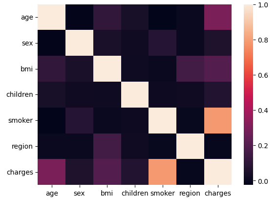
Figure 1. Multicollinearity of the dataset

To better deal with the dataset, categorical value like sex, smoker and region are converted to numeric data. For sex and smoker, they are converted to simple 0s and 1s to distinguish whether an insurer is male or female, smoker or non-smoker. For regions, there are a total of four different categories: northeast, southeast, southwest, and northwest. They are converted to 0 to 3 to each represent a region.

After the dataset is preprocessed, a heat map, in figure 1, is made to check the multicollinearity of the dataset. It is clear that independent variables do no show significant correlation with each other, which means the MLR model will be more accurate. As result, the author will select all variables to construct an MLR model.

It is also shown in figure 1 that age, bmi, and smoker are more correlated with charges, and the correlations between each independent variables and the dependent variable will be explained in the result section.

3.3. Linear regression method

The linear regression function can be simplified to its basic form of a regression line: \( {f_{w,b}}(x)=wx+b→\hat{y} \) where w is slope and b is intercept. To find the optimal w and b, it is important to minimize the mean square error (MSE): \( \frac{1}{n}\sum _{i=1}^{n}{({f_{w,b}}({x_{i}})-{y_{i}})^{2}} \) which penalize poor estimations. Before minimizing the MSE, variables x, w, and y should be written in vector form. \( x=(\begin{matrix}1 & … & {x_{1}} \\ 1 & … & {x_{i}} \\ 1 & … & {x_{N}} \\ \end{matrix})=(\begin{matrix}{x_{10}} & {x_{11}} & … & {x_{1D}} \\ {x_{i0}} & {x_{11}} & … & {x_{iD}} \\ {x_{N0}} & {x_{N1}} & … & {x_{ND}} \\ \end{matrix}) \) \( w=(\begin{matrix}{w_{0}}=b \\ … \\ {w_{D}} \\ \end{matrix}) \) , and \( y=(\begin{matrix}{y_{1}} \\ … \\ {y_{n}} \\ \end{matrix}) \) . Now, the MSE can be minimized by setting its partial derivative to zero with respect to \( {w_{k}} \) for k from 0 to D.

\( \frac{∂y}{∂{w_{k}}}(MSE)=\frac{1}{N}\sum _{i=1}^{N}2({y_{i}}-\sum _{j=0}^{D}{w_{j}}{x_{ij}})(-{x_{ik}})=0 → \sum _{i=1}^{N}{y_{i}}{x_{ik}}=\sum _{i=1}^{N}\sum _{j=0}^{D}{w_{j}}{x_{ij}}{x_{ik}} \\ → \sum _{i=1}^{N}X_{ki}^{T}{y_{i}}=\sum _{j=0}^{D}(\sum _{i=1}^{n}X_{ki}^{T}{x_{ij}}){w_{j}} → {[{X^{T}}y]_{k}}={[({X^{T}}X)w]_{k}} → w={({X^{T}}X)^{-1}}{X^{T}}y \ \ \ (1) \)

4. Results and discussion

4.1. Descriptive analysis

Figure 2 contains two histograms that each shows the distribution of medical insurance charges for smoker and non-smoker.

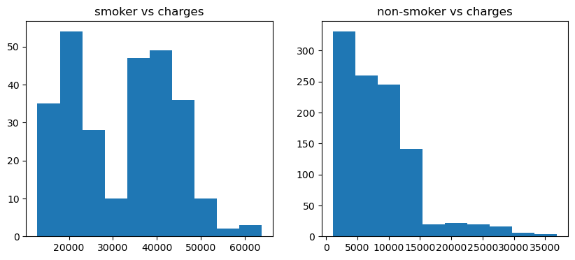
Figure 2. Distribution of changes for smoker and non-smoker

From figure 3, it is clear that people with smoking behavior tend to spend more on insurances charges while people who do not smoke spend much less. It is a strong indicator that smoking is highly correlated with worse health conditions that tend to incur high charges. It is also worth noticing that gender is not an important factor in influencing the insurance charges. As the violin plot figure 4 shows below, the shape of the plots is relatively same for both male (as sex 0 in figure 3) and female (as sex 1), showing that the distribution of charges is also similar for both sexes. The only factor that causes the plots to be different is smoking. It is clear that smoking induces a higher insurance charge no matter it is male or female, and smoking causes women to pay more than men.

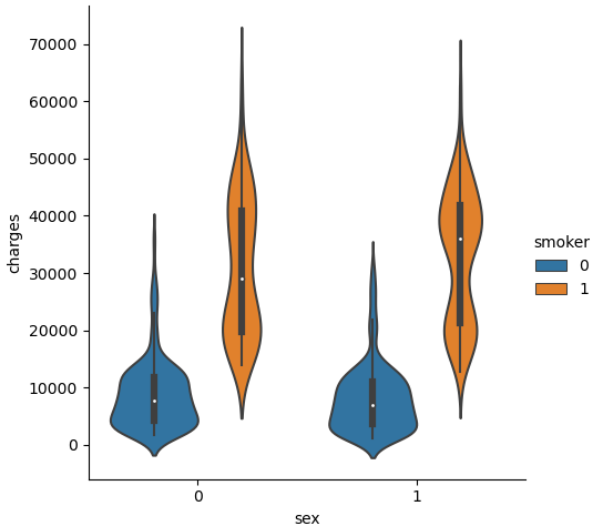
Figure 3. Distribution of charges for male, female, distinguished by smoking behavior

Figure 4 below shows the distribution of charges for different ages. For non-smoking insurers, it is clear that the charges remain low and increase steadily with growing age. However, for smoking insurers, although the charges also increase steadily, they are much higher than non-smokers. It is also remarkable that the plot for smokers has two stripes of dots. This is relevant to figure 4 which shows the width of the violin graph is wider for smoking women at higher charged than men. It is likely that the higher strip of dots represents smoking women and the lower strip of dots represent smoking men. It is also assumed that smokers have a higher tendency of developing other unhealthy behaviors that subsequently increase the insurance charges.

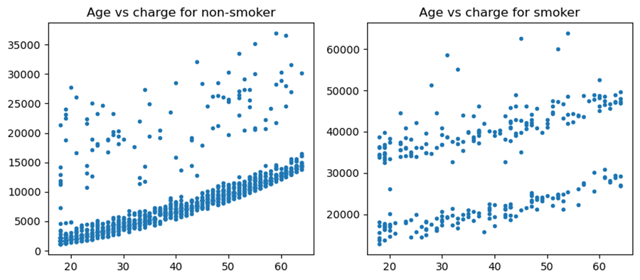
Figure 4. Distribution of charges for different ages, distinguished by smoking behavior

Figure 5 shows the correlation between body mass index (bmi) and charges. A bmi over 30 is often considered obese which has greater potentials of inducing serious diseases [6]. The graph shows that for non-smokers, insurance charges only increase slightly as their bmi increases. However, for smokers, the insurances charges increase dramatically with the rising of bmi. This can potentially explain why there are two stripes of points in the second plot of figure 5.

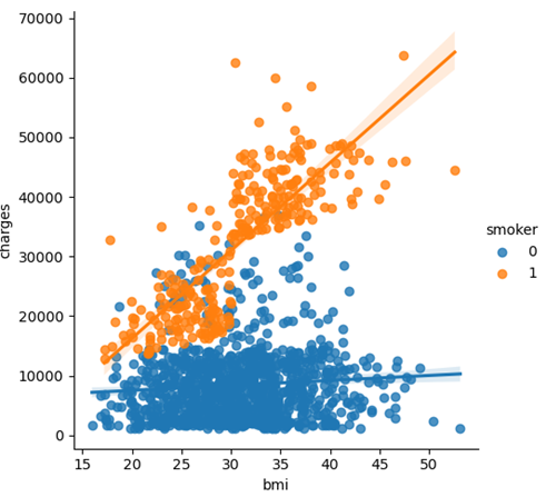
Figure 5. Distribution of charges for different bmi, distinguished by smoking behavior

Figure 6 and 7 below shows the histogram of the number of children that insurers have and the correlation between number of children and medical insurances charges. The histogram shows that the number of insures decreases as the number of children that have increases. It shows that most insurers have 1 and less children. The second violin graph shows the relationship between charges and number of children. It is clear that they only possess a weak correlation since the shape of the violin is almost identical across the number of children, with the only exception of children number 4 and 5 due to lack of samples.

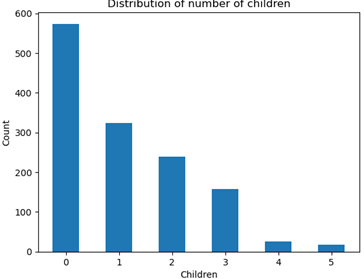
Figure 6. Distribution of number of children

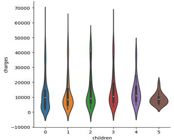
Figure 7. Correlation between number of children and charges

Although number of children only possess a weak correlation with charges, it may not be a wise idea to drop this variable from the MLR model as Rossi et al. suggest in their paper [4]. Therefore, the author decides to include all variables for the MLR model. In the end, the author uses Python’s scikit-learn to make the MLR model:

\( charge=-11815.45+257.29*age-131.11*sex+…-353.64*region.\ \ \ (2) \)

From this MLR model, it is evident that smoking is the most correlated variable with a large coefficient of 23820.43. It is clear that smoking deteriorates health condition which in turn prompts insurances companies to charge a higher price. It is notable that sex has the weakest correlation with the insurance charges. The model shows that sex is not an important factor that determines the insurance charges. An unexceptional outcome is that bmi is also weakly correlated with charges, given the fact that higher bmi leads to worse health condition (table 2).

Table 2. MLR Results

Lastly, the author uses the score function of scikit-learn to obtain the R-Squared score of this MLR model. The score is estimated to be 0.75, which is considered a successful attempt.

5. Conclusion

In this paper, the author conducts an exploratory analysis on medical insurance dataset from Kaggle. The author preprocesses the dataset at first and shows the correlation between each independent variable and the dependent variable. In the end, the author provides the MLR model with a satisfactory accuracy of 0.75.

It cannot be denied that overfitting may be a problem for this dataset since it contains only around 1000 inputs. More data should be incorporated to prevent this issue in future studies. Other prediction models like Random Forest can also be incorporated in future studies to compare with MLR in order to achieve a better prediction result.

References

[1]. James W, et al. 2004 Overweight and Obesity (High Body Mass Index). Comparative Quantification of Health Risks: Global and Regional Burden of Disease Attributable to Selected Major Risk Factors, 497-596.
[2]. Tranmer M, Murphy J, Elliot M and Pampaka M 2020 Multiple Linear Regression (2nd Edition). Cathie Marsh Institute, Working Paper, 1.
[3]. Joshua C 2023 Implementing Multiple Linear Regression model using Neural Networks. ResearchGate.
[4]. Gülden K U and Neşe G A 2013 Study on Multiple Linear Regression Analysis. Procedia - Social and Behavioral Sciences, 234-240.
[5]. Elena R, Isabella P and Renato I 2022 Multilinear Regression Model for Biogas Production Prediction from Dry Anaerobic Digestion of OFMSW. Sustainability 14, 4393.
[6]. Smita R, Alakananda T and Alok R T 2020 Prediction of new active cases of coronavirus disease (COVID-19) pandemic using multiple linear regression model. Diabetes & Metabolic Syndrome: Clinical Research & Reviews, 14(5), 1467-1474.
[7]. Knofczynski G T and Mundfrom D 2007 Sample Sizes When Using Multiple Linear Regression for Prediction. Educational and Psychological Measurement, 68(3), 431-442.
[8]. Stephen Y, et al. 2018 Predicting Students' Academic Performance Using Multiple Linear Regression and Principal Component Analysis, Journal of Information Processing.
[9]. Stavroula D and Konstantinos G N 2022 Multiple Linear Regression Models with Limited Data for the Prediction of Reference Evapotranspiration of the Peloponnese, Greece. Hydrology, 9, 124.
[10]. Biau G and Scornet E 2016 A random forest guided tour. TEST, 25, 197-227.
Cite this article
Dai,W. (2024). Predicting insurance charges using linear regression models. Theoretical and Natural Science,51,51-57.
Data availability
The datasets used and/or analyzed during the current study will be available from the authors upon reasonable request.
Disclaimer/Publisher's Note
The statements, opinions and data contained in all publications are solely those of the individual author(s) and contributor(s) and not of EWA Publishing and/or the editor(s). EWA Publishing and/or the editor(s) disclaim responsibility for any injury to people or property resulting from any ideas, methods, instructions or products referred to in the content.
About volume
Volume title: Proceedings of CONF-MPCS 2024 Workshop: Quantum Machine Learning: Bridging Quantum Physics and Computational Simulations
© 2024 by the author(s). Licensee EWA Publishing, Oxford, UK. This article is an open access article distributed under the terms and
conditions of the Creative Commons Attribution (CC BY) license. Authors who
publish this series agree to the following terms:
1. Authors retain copyright and grant the series right of first publication with the work simultaneously licensed under a Creative Commons
Attribution License that allows others to share the work with an acknowledgment of the work's authorship and initial publication in this
series.
2. Authors are able to enter into separate, additional contractual arrangements for the non-exclusive distribution of the series's published
version of the work (e.g., post it to an institutional repository or publish it in a book), with an acknowledgment of its initial
publication in this series.
3. Authors are permitted and encouraged to post their work online (e.g., in institutional repositories or on their website) prior to and
during the submission process, as it can lead to productive exchanges, as well as earlier and greater citation of published work (See
Open access policy for details).