1 Introduction

With the rise of computers and increasing computational power, the field of Computational Fluid Dynamics (CFD) has become a common tool for predicting the real flow. CFD, is the process of using computational power to make mathematical predictions about physical fluid flow by solving the governing equations. In CFD methods used in present, Reynolds-Averaged Navier-Stokes (RANS) has become the most popular method in engineering for its low cost and acceptable accuracy of simulation.

During past decades, many researched has proposed lots of turbulence models to close RANS equations. For example, Launder proposed standard \( k-ϵ \) model in 1974^[1] and Wilcox developed \( k-ω \) model in 1988[2], which are commonly used even today. However, the parameters in turbulence models introduce uncertainties into calculation, for the parameters are often set with several typical experiments, which can’t represent all types of flow. Therefore, it is meaningful to explore the effect of parameters on calculations of flow, i.e. parametric uncertainty.

Research about parametric uncertainty can guide the calibration of turbulence models. Cheung[3] used Bayesian method to investigate parametric uncertainty of the S-A model, and calibrated the parameters with friction coefficients and velocity data, Chowdhary [4] discovered the inherent defect of the SST model when exploring parametric uncertainty based hypersonic turbulence flow experiment. These research all proved the necessity to learn about how parameters affect calculation results of turbulence models. Therefore, this research focuses on the effect of the generalized \( k-ω \) (GEKO) two-equation turbulence model on backward facing step, which is a typical case to test the performance of turbulence model in simulating separated flow.

In general, this research will be divided into 4 sections. In the second part, methods used are illustrated. In Section 3, calculation details of the backward facing step are displayed. After completing the previous steps, the results will be analyzed. Finally, conclusion is drawn based on the results.

2 Method

2.1 Governing equations

There are three governing equations, which represent mass, momentum and energy conservation respectively:

\( \begin{cases}&\frac{∂ρ}{∂t}+\frac{∂}{∂x_{j}}(ρu_{j})=0 \\&\frac{∂(ρu_{i})}{∂t}+\frac{∂}{∂x_{j}}(ρu_{i}u_{j})=-\frac{∂P}{∂x_{i}}+\frac{∂}{∂x_{j}}(τ_{ij}+τ_{ij}^{t}) \\&\frac{∂(ρE)}{∂t}+\frac{∂}{∂x_{j}}(ρHu_{j})=\frac{∂}{∂x_{j}}[u_{i}(τ_{ij}+τ_{ij}^{t})+(\frac{μ}{Pr_{1}}+\frac{μ_{t}}{Pr_{t}})\frac{∂h_{s}}{∂x_{j}}] \end{cases},\ \ \ (1) \)

where \( ρ \) is the fluid density, \( u_{i} \) represents the velocity vector in \( x_{i} \) direction, \( P \) is the pressure, \( τ_{ij} \) and \( τ_{ij}^{t} \) are the molecular stress tensor component and the Reynolds stress tensor component respectively, \( μ \) and \( μ_{t} \) are the molecular viscosity and the turbulent eddy viscosity respectively, \( Pr_{1} \) and \( Pr_{t} \) are the laminar and turbulent Prandtl number respectively, and \( h_{s} \) is the specific enthalpy. \( E \) and \( H \) are the total energy and enthalpy, which can be written as:

\( E=e+\frac{u_{i}u_{i}}{2},\ \ \ (2) \)

\( H=E+\frac{P}{ρ},\ \ \ (3) \)

where \( e \) is the specific internal energy.

2.2 The generalized \( k-ω \) two-equation turbulence model

The GEKO turbulence model is proposed by Mentor[5]. The model formulation is given by:

\( \frac{∂(ρk)}{∂t}+\frac{∂(ρU_{j}k)}{∂x_{i}}=-τ_{ij}\frac{∂U_{i}}{∂x_{j}}-C_{μ}ρkω+\frac{∂}{∂x_{j}}[(μ+\frac{μ_{t}}{σ_{k}})\frac{∂k}{∂x_{j}}],\ \ \ (4) \)

\( \frac{∂(ρω)}{∂t}+\frac{∂(ρU_{j}ω)}{∂x_{j}}=C_{ω1}F_{1}\frac{ω}{k}P_{k}-C_{ω2}F_{2}ρω^{2}+ρF_{3}CD+\frac{∂}{∂x_{j}}[(μ+\frac{μ_{t}}{σ_{ω}})\frac{∂ω}{∂x_{j}}],\ \ \ (5) \)

with

\( μ_{t}=ρv_{t}=ρ\frac{k}{max{(ω,\frac{S}{C_{Realize}})}},\ \ \ (6) \)

\( C_{Realize}=\frac{1}{\sqrt[]{3}},\ \ \ (7) \)

\( CD=\frac{2}{σ_{ω}}\frac{1}{ω}\frac{∂k}{∂x_{j}}\frac{∂ω}{∂x_{j}}.\ \ \ (8) \)

The main characteristic of the GEKO model is that it has several additional parameters. These free parameters can be adjusted to cover a wide range of flow variations, and they are embedded through the functions \( F_{1} \) , \( F_{2} \) and \( F_{3} \) in the above equations. Parameters added in the GEKO model are designed to control specific physical aspects of the model, including near wall behavior, separation, free jet dynamics and so on. In this research, we selected three important parameters \( C_{sep},C_{nw}, C_{jet} \) .

2.3 The prior range of the parameters

To ensure the convergence of calculations, we set the limit of the prior range of parameters as \( ±25% \) of the nominal value. The prior range of \( C_{sep},C_{nw}, C_{jet} \) is listed in Table 1.

Table 1. The range of parameters of \( k-ω \) GEKO model

In the experiment, the Latin hypercube sampling is chosen to be the method to calculate data. Latin hypercube is a random sampling technique designed to reduce the correlation between input variables and thus improve the accuracy of Monte Carlo simulations. It ensures the randomness and homogeneity of the samples by dividing the range of values of each component equally into equal intervals and randomly selecting a value within each interval. The sampling number \( K \) can be calculated by[6]:

\( K=\frac{(n+p)!}{n!p!}×n_{p}\ \ \ (9) \)

where \( n \) is the number of parameters, \( p \) is the polynomial chaos number, and \( n_{p} \) is oversampling ratio. In this paper, with \( n=3 \) , \( p=2 and n_{p}=2, \) we can obtain \( K=20. \)

3 Simulation details

As one of the simplest and most typical two-dimensional separated flow, the backward facing step[7] has been universally emphasized and tested. The geometry shape of the experiment is shown in Fig. 1, where \( H=1.27cm \) is the height of the step and \( U_{ref} \) is the reference velocity at the inlet.

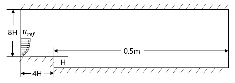
Figure 1. Geometry shape of the backward facing step

The grid will influence the accuracy of the simulation. To avoid the effect of grids, grid Reynolds number is set as \( y^{+} \lt 1 \) . The scheme of the grid is shown in Fig. 2.

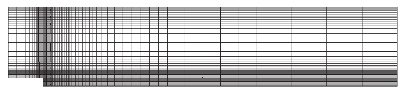
Figure 2. The scheme of the grid of the backward facing step

To ensure that the velocity distribution upstream the step is consistent with the experiment, the boundary type of the inlet is chosen as the velocity inlet. Detailed inlet conditions are shown in Table 2. The wall is set as adiabatic wall. The SIMPLEC algorithm is used, the second-order upwind format is adopted. Calculations are conducted with Fluent. All simulations are converged.

Table 2. Inlet conditions of the simulation

4 Analysis and discussion

4.1 Normal calculation

Firstly, the calculation is done with nominal values of the parameters. The contour of the velocity is shown in Fig. 3. It can be seen that the boundary layer starts to separate at the edge of the step, and backflow occurs in the separation area downstream of the step. The separation area is mainly concentrated in the triangle area from the step to the reattachment point, and the boundary of the separation area is clear. Then the boundary layer continues to develop in the downstream boundary layer of the separation zone until the exit.

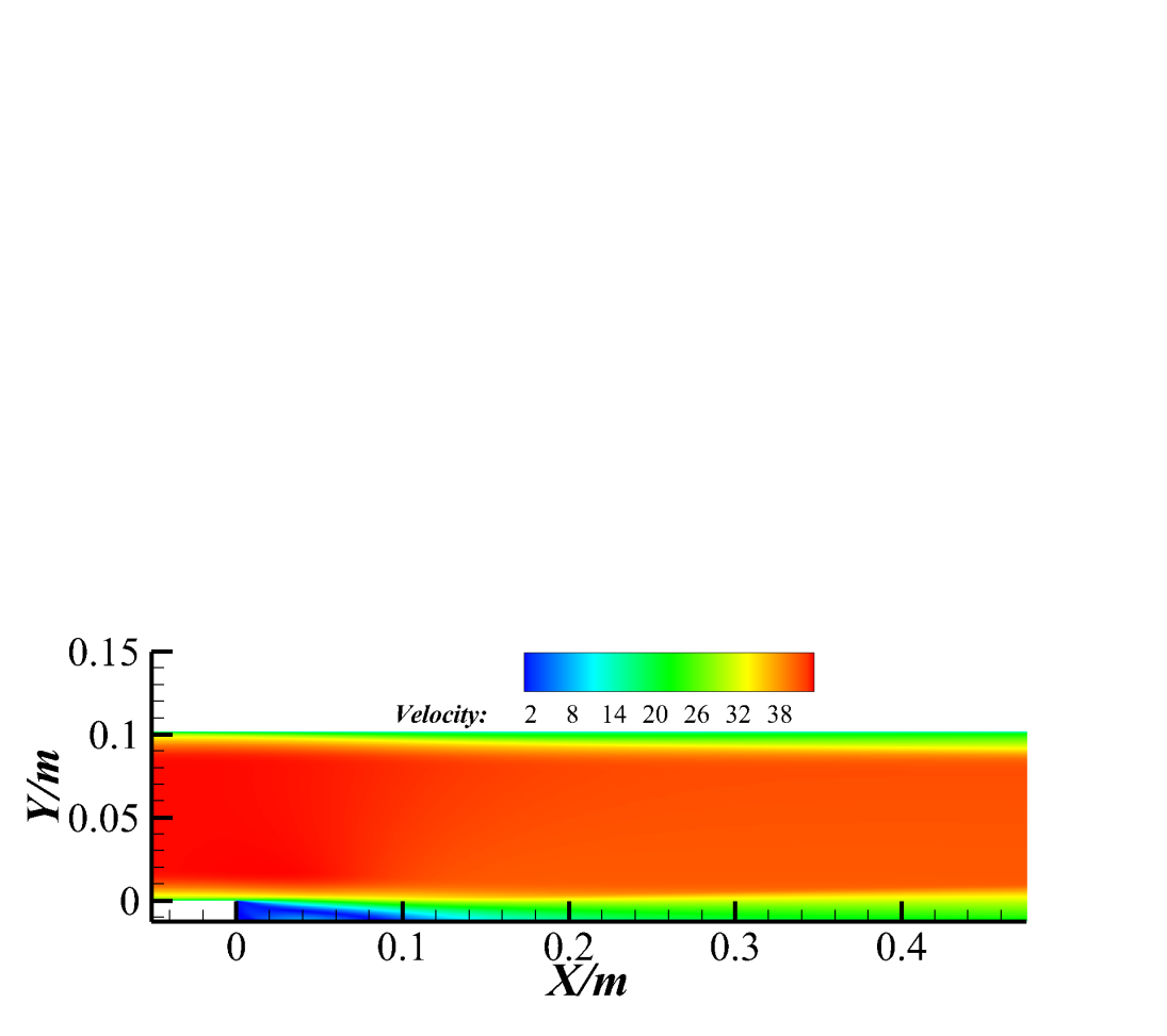
Figure 3. The contour of the velocity for backward facing step with nominal parameters

4.2 Prior analysis

Prior results calculated with 20 sets of parameters are shown in Fig. 4. It can be seen that the results obtained by using the nominal values of the parameters are within the prior range. The pressure coefficient of the separation zone, recovery zone and development zone has little change with the original parameter value after the change of parameters, and generally cannot cover the experimental value, which means that the change of three parameters cannot make up for the defects of the model itself. For the friction coefficient, changing the parameters’ values significantly affects the calculation results. More experimental points are covered, indicating that calibrating the model parameters may improve the friction coefficient better than the pressure coefficient.

(a) \( C_{p} \)	(b) \( C_{f} \)

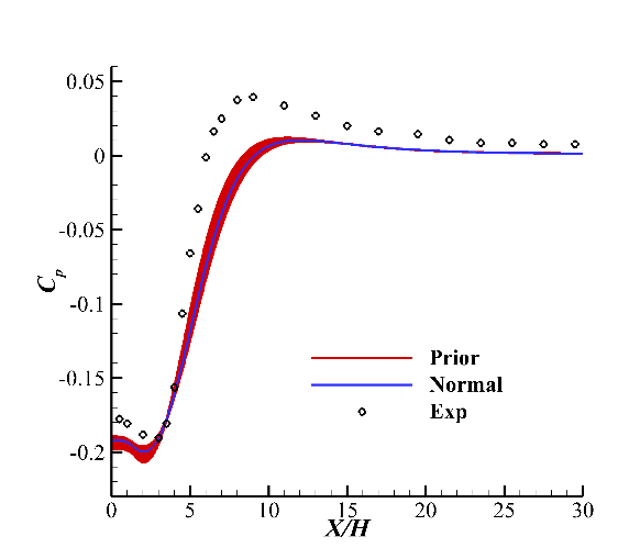
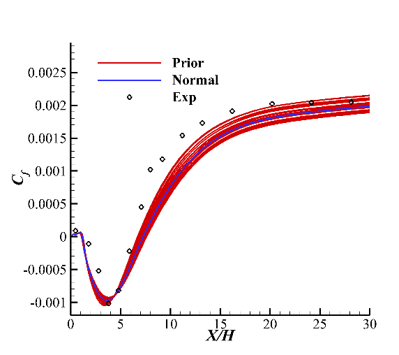
Figure 4. Prior results calculated with 20 set of parameters

We can obtain the sensitivity index of each parameter by constructing polynomials, that is, the Sobol index. We can decompose a variable into a sum of polynomials as

\( α^{*}(X,ξ)≈\sum_{j=0}^{P} α_{j}(X)Ψ_{j}(ξ),\ \ \ (10) \)

where \( α^{*}(X,ξ) \) is the value of the variable calculated with the parameter \( ξ \) at location of \( X \) . The mean \( μ \) and variance \( D \) of the variable can be given by

\( μ=α_{0}(x), \\D=\sum_{i=1}^{P} α_{i}^{2}(x)⟨Ψ_{i}^{2}(ξ)⟩. \ \ \ (11) \)

According to Crestaux et al.[8], \( D \) can be split into

\( \begin{cases}&D=\sum_{i=1}^{i=n} D_{i}+\sum_{1≤i \lt j≤n}^{i=n-1} D_{i,j}+\sum_{1≤i \lt j \lt k≤n}^{i=n-2} D_{i,j,k}+…+D_{1,2,…,n}, \\&D_{i_{1},…,i_{s}}=\sum_{β∈(i_{1},…,i_{s})}^{} α_{β}^{2}⟨Ψ_{β}^{2}(ξ)⟩,1≤i \lt … \lt i_{s}≤n. \end{cases}\ \ \ (12) \)

Then the Sobol index can be given by

\( S_{i_{1}…i_{s}}=\frac{D_{i_{1}…i_{s}}}{D}.\ \ \ (13) \)

The Sobol indices of three parameters for the pressure coefficient and friction coefficient are shown in Fig. 5. As can be seen, the sensitivity of \( C_{sep} \) dominates whether the results of \( C_{p} \) and \( C_{f} \) , which clearly proved the important effect of the construction of \( C_{sep} \) . For \( C_{p} \) , in the separation zone, the Sobol indices of \( C_{nw} \) and \( C_{jet} \) is extremely low. While after the reattachment point, the sensitivity of \( C_{nw} \) and \( C_{jet} \) begin to increase. For \( C_{f} \) , the sensitivity is chaos near the step, which is caused by the appearance of the corner vortex. In other region, the sensitivity of \( C_{jet} \) maintains low, while the sensitivity of \( C_{nw} \) recovers downstream.

(a) \( C_{p} \)	(b) \( C_{f} \)

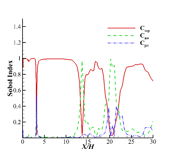
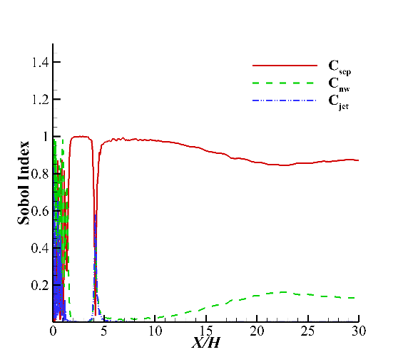
Figure 5. Sobol indices of three parameters for \( C_{p} \) and \( C_{f} \)

The Sobol indices of three parameters for the location of reattachment point are shown in Fig. 6. \( C_{nw} \) is the most sensitive parameter and the sensitivity of \( C_{sep} \) and \( C_{jet} \) are similar. This is not very surprising because increasing \( C_{nw} \) leads to higher wall shear stress in non-equilibrium flows, which will directly affect the location of the reattachment point.

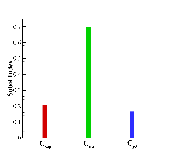
Figure 6. Sobol indices of three parameters for the location of reattachment point

The values of the parameters and the reattachment point are listed in Table 3. From the table. We can see that there are 9 sets of calculations which give less relative error of the reattachment point than with nominal values of the parameters. For these samples, the denominator is that they all have small \( C_{sep} \) , which means that although the Sobol index of \( C_{sep} \) is not the biggest, it plays an important role in the process of reattachment. By decreasing \( C_{sep} \) , eddy-viscosity is decreased too, which leads to more sensitivity to adverse pressure gradients for boundary layers and lower spreading rates for free shear flows. This results in a smaller separation zone.

Table 3. The values of the parameters and the reattachment point

The relative error calculated with 20 sets of parameters for \( C_{p} \) and \( C_{f} \) is listed in Table 4. We can see that the calculation of the reattachment point is positively correlated with the calculation of \( C_{p} \) and \( C_{f} \) to some extent. That is to say, the samples with a better calculated reattachment point also have better calculated \( C_{p} \) and \( C_{f} \) , although this doesn’t mean that better \( C_{p} \) will lead to better \( C_{f} \) . Besides, a better calculated reattachment point tends to better \( C_{f} \) . This is because the correlation between the reattachment point and \( C_{f} \) : The reattachment point is the location where \( C_{f} \) equals to zero. All in all, considering the three variables we obtained, \( C_{sep}=1.3125 \) , \( C_{nw}=0.4675 \) and \( C_{jet}=0.52 \) (Set 8) lead the best results.

Table 4. The relative error calculated with 20 sets of parameters for \( C_{p} \) and \( C_{f} \)

5 Conclusions

In a nutshell, we conduct calculations with different values of parameters of the GEKO turbulence model based on backward facing step flow. With Latin hypercube sampling, parameters are obtained in the form of a uniform distribution. Then the prior range of the pressure coefficient and friction coefficient and the sensitivity of parameters is analyzed. At the same time, the calculation error of the reattachment point is compared. Some conclusions are drawn:

1 \( C_{sep} \) plays an important role in the calculations of separation, especially for the pressure coefficient and friction coefficient. \( C_{nw} \) dominates the simulation of the reattachment point, which is because \( C_{nw} \) directly affects eddy-viscosity.

2 The calculation of the reattachment point, \( C_{p} \) and \( C_{f} \) appears to be correlated that a better reattachment point will lead to better calculated \( C_{p} \) and \( C_{f} \) . Better \( C_{p} \) doesn’t mean better \( C_{f} \) , but a better reattachment point often corresponds to better \( C_{f} \) .

3 A smaller \( C_{sep} \) will lead to a smaller separation zone, which results in the increase of calculation accuracy for backward facing step. \( C_{sep}=1.3125 \) , \( C_{nw}=0.4675 \) and \( C_{jet}=0.52 \) (Set 8) will lead to a better result for backward facing step.

References

[1]. Launder, Brian Edward, and Bahrat I. Sharma. "Application of the energy-dissipation model of turbulence to the calculation of flow near a spinning disc." Letters in heat and mass transfer 1.2 (1974): 131-137.
[2]. Wilcox, David C. "Reassessment of the scale-determining equation for advanced turbulence models." AIAA journal 26.11 (1988): 1299-1310.
[3]. Cheung, Sai Hung, et al. "Bayesian uncertainty analysis with applications to turbulence modeling." Reliability Engineering & System Safety 96.9 (2011): 1137-1149.
[4]. Chowdhary, Kenny, et al. "Calibrating hypersonic turbulence flow models with the HIFiRE-1 experiment using data-driven machine-learned models." Computer Methods in Applied Mechanics and Engineering 401 (2022): 115396.
[5]. Menter, F.R., Matyushenko, A. and Lechner, R., "Development of a Generalized k-ω (GEKO) Two-Equation Turbulence Model", presented at the 21st DGLR-Fach-Symposium der STAB, Darmstadt, Germany (2018)
[6]. Hosder, Serhat, Robert W. Walters, and Michael Balch. "Point-collocation nonintrusive polynomial chaos method for stochastic computational fluid dynamics." AIAA journal 48.12 (2010): 2721-2730.
[7]. Driver, David M., and H. Lee Seegmiller. "Features of a reattaching turbulent shear layer in divergent channelflow." AIAA journal 23.2 (1985): 163-171.
[8]. Crestaux, Thierry, Olivier Le Maıtre, and Jean-Marc Martinez. "Polynomial chaos expansion for sensitivity analysis." Reliability Engineering & System Safety 94.7 (2009): 1161-1172.
Cite this article
Hu,Y. (2024). Investigation of the effect of three parameters in the GEKO model on the calculation results for backward facing step flow. Theoretical and Natural Science,56,32-39.
Data availability
The datasets used and/or analyzed during the current study will be available from the authors upon reasonable request.
Disclaimer/Publisher's Note
The statements, opinions and data contained in all publications are solely those of the individual author(s) and contributor(s) and not of EWA Publishing and/or the editor(s). EWA Publishing and/or the editor(s) disclaim responsibility for any injury to people or property resulting from any ideas, methods, instructions or products referred to in the content.
About volume
Volume title: Proceedings of the 2nd International Conference on Applied Physics and Mathematical Modeling
© 2024 by the author(s). Licensee EWA Publishing, Oxford, UK. This article is an open access article distributed under the terms and
conditions of the Creative Commons Attribution (CC BY) license. Authors who
publish this series agree to the following terms:
1. Authors retain copyright and grant the series right of first publication with the work simultaneously licensed under a Creative Commons
Attribution License that allows others to share the work with an acknowledgment of the work's authorship and initial publication in this
series.
2. Authors are able to enter into separate, additional contractual arrangements for the non-exclusive distribution of the series's published
version of the work (e.g., post it to an institutional repository or publish it in a book), with an acknowledgment of its initial
publication in this series.
3. Authors are permitted and encouraged to post their work online (e.g., in institutional repositories or on their website) prior to and
during the submission process, as it can lead to productive exchanges, as well as earlier and greater citation of published work (See
Open access policy for details).