1 Introduction

Monte Carlo methods are used widely in the field of finance, biology, physical sciences and engineering. Its core advantage lies in its ability to handle complex randomness and uncertainty problems, providing more accurate basis for decision-making. However, it also has many drawbacks including high computational costs, slow convergence speed, large sample size requirements, and high dependence on the model. Therefore, to estimate intervals accurately and efficiently, variance reduction is crucial. This paper explores a new numerical integration method called splitting method for reducing intrinsic variance in Monte Carlo simulations. The application of these techniques not only optimizes computing resources but also broadens the applicability of Monte Carlo methods. The paper is divided into five parts: the first part is the introduction of the paper, the second part reviews related work of the applications of Monte Carlo methods in different fields, the third part describes Monte Carlo methods and control variates, the fourth part presents experimental results of various functions and proposes the innovative method, and the fifth part draws conclusions and discusses the limitation of this paper.

2 Literature Review

Nowadays, Monte Carlo methods are usually applied in the fields of mathematics and science and can effectively solve various complicated mathematical problems. Maanane et al. used the symbolic Monte Carlo method to identify the radiation characteristics of non-uniform materials, and the polynomials obtained through this method allow for complete inverse analysis, thereby improving efficiency and stability [1]. Meanwhile, Zhou et al. introduced the Monte Carlo method in the stability analysis of the dispersion strength characteristics of soil rock mixtures, effectively improving the accuracy of the stability analysis method [2]. Wicaksono et al. proposed a new paradigm Monte Carlo Fuzzy Hierarchy Analysis (NMCFAHP) by introducing normally distributed fuzzy numbers, which is more effective in overcoming uncertainty in the group decision-making process [3]. In addition, Sangwongwanich et al. developed a Monte Carlo simulation method with incremental damage by considering the cumulative damage of the system, which is suitable for fault-tolerant systems and can be effectively applied in the direction of reliability assessment of power electronic equipment [4]. Moreover, Mongwe et al. proposed a new method for solving the high variance problem in Hamiltonian Monte Carlo (HMC) estimators, including back sampling combined with importance sampling, diamagnetic Hamiltonian Monte Carlo, and diamagnetic momentum Hamiltonian Monte Carlo, to improve posterior inference in machine learning [5]. Afterwards, Sarrut et al. reviewed the ecosystem of the open-source Monte Carlo toolkit GATE for medical physics and introduced the application of Monte Carlo simulation methods in medical physics [6]. Besides, Song et al. provided a more comprehensive exposition of Monte Carlo and variance reduction methods, a thorough review of the relevant formulations and techniques, and an in-depth summary of the development of existing numerical methods, covering general formulations, specific subcategories and their variants, and applications, as well as a comparison of the strengths and weaknesses of different methods [7]. Furthermore, considering the uncertainty of out-of-distribution data prediction, Yelleni et al. proposed the Monte Carlo DropBlock (MC DropBlock) method to simulate the uncertainty in YOLO and the convolutional visual transformer used for object detection, effectively improving the model's generalization ability [8]. And Mazzola, G also analyzed the feasibility of Monte Carlo’s application in the field of quantum computing and the future challenges it faces [9]. Monte Carlo methods have already been applied in so many fields, so it is of great practical significance to improve the precision of Monte Carlo methods through variance reduction.

3 Methods

3.1 Monte Carlo Methods

In many applications in mathematics, computing the expectation \( E[X] \) of a random variable X, e.g., in option pricing or utility maximization theory is often needed. However, it is not always possible to compute \( E[X] \) analytically. Therefore, it is crucial to find methods to approximate).

Suppose there is a sequence of random variables ( \( X_{i} \) ), which are mutually independent and identically distributed with the same distribution as X. Then, with probability one, we have

\( \frac{1}{n}\sum_{i=1}^{n} X_{i} → E[X], (n→∞). (1) \)

by the so-called Strong Law of Large Numbers (SLLN), which turns a sequence of random observations into a deterministic number by computing the average.

If many independent realizations are generated from the same distribution, and these realizations are averaged, by the SLLN, it is sure that for large n the average is close to the true expected value, which is called Monte Carlo methods. Monte Carlo methods stem from the analogy between probability and volume and calculate the volume of a set by interpreting the volume as a probability. In the simplest case, this means randomly sampling from a range of possible outcomes and selecting a portion from a given set as an estimate of the volume of that set. The law of large numbers ensures that as the number of draws increases, the estimate value will converge to the correct value. The central limit theorem provides information on the possible size of estimation errors after finite drawing [10].

Monte Carlo method algorithms can be summarized as the following pattern:

1.Define a possible input domain

2.Generate inputs randomly based on the probability distribution on the domain

3.Perform a deterministic calculation of the outputs

4.Sum up the results

In principle, Monte Carlo methods can be used to solve any problem with probabilistic explanations. However, a major limitation of Monte Carlo methods is their high dependence on sample size. For example, let's evaluate \( \int_{0}^{1} x^{2}dx. \)

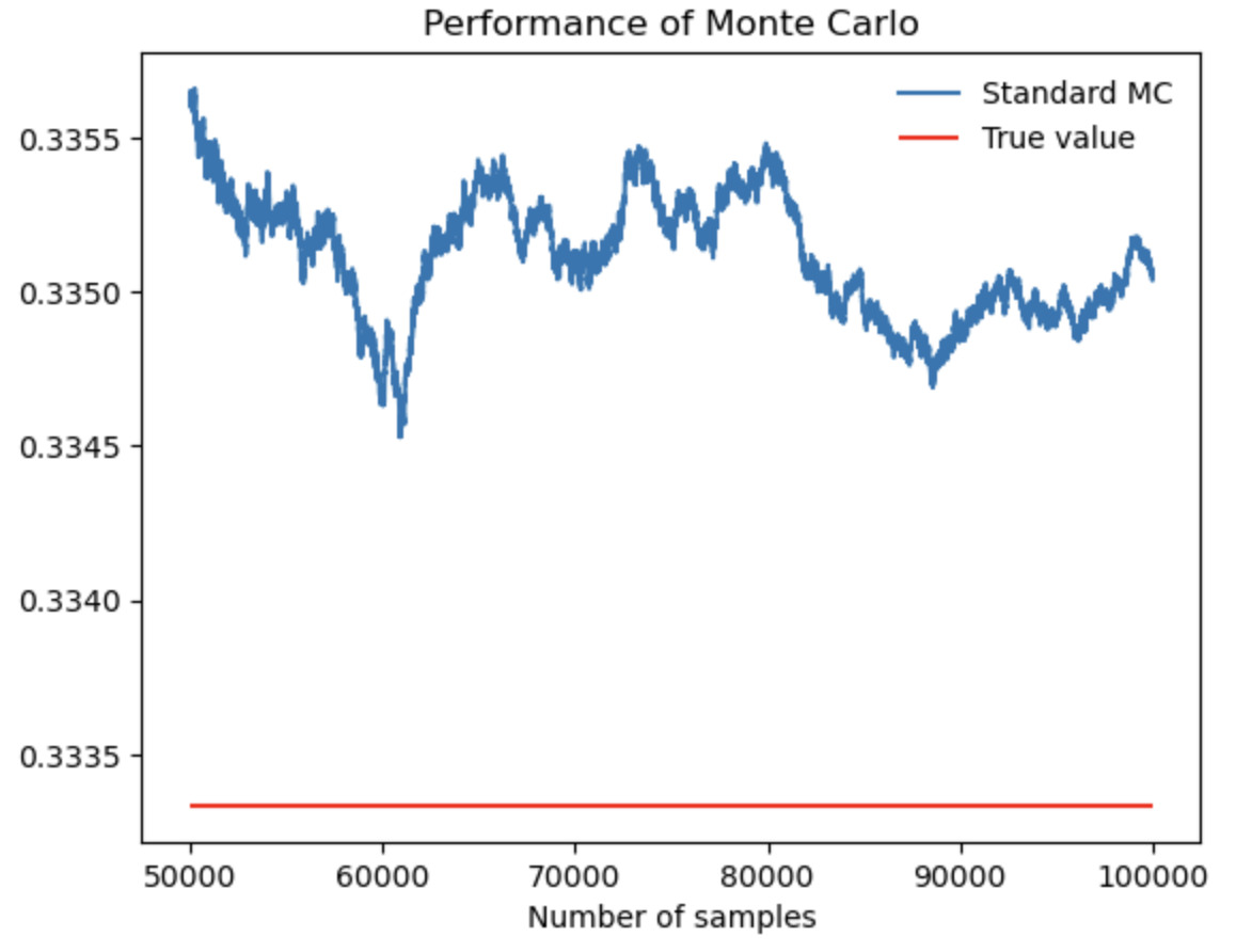
Figure 1. Performance of Monte Carlo when evaluate \( \int_{0}^{1} x^{2} \) .

As figure 1 shows, even if the sample size in Monte Carlo simulation is large enough, it is impossible to estimate a perfect fit with the correct value because the accuracy of Monte Carlo estimation is limited by the random distribution and integral characteristics of the samples.

3.2 Control Variates

The method of control variates is one of the most effective and widely applicable techniques to improve the efficiency of Monte Carlo simulations. It utilizes the information of known quantity estimation error to realize error decreasing of unknown quantity estimation [10].

The control-variates method for estimating \( E[X] \) can be described as follows.

Suppose the pairs ( \( X_{i} \) , \( Y_{i} \) ), i = 1, . . ., n are independent and identically distributed, and that the expectation E[Y] is known. The control-variates estimator with b* of \( E[X] \) is defined by

\( \bar{X_{n}}(b) \bar{X_{n}} - b(\bar{Y_{n}}- E[Y]) = \frac{1}{n}\sum_{i=1}^{n} (X_{i}- b(Y_{i} - E[Y])) (2) \)

Note that the observed error \( \bar{Y}_{n} \) - \( E[Y] \) is used to control the estimation of E[X].

The mean of the control-variates estimator is

\( E[\bar{X_{n}}(b)]= \frac{1}{n}\sum_{i=1}^{n} E[X_{i}(b)] = E[X], (3) \)

so, it's unbiased. The variance of the control-variates estimator is

\( Var(\bar{X_{n}}(b)) = \frac{1}{n^{2}}\sum_{i=1}^{n} Var(X_{i}(b)) (4) \)

\( = \frac{1}{n}Var(X_{i}(b)) (5) \)

\( = \frac{1}{n}(Var(X)-2bCov(X,Y)+b^{2} Var(Y)) (6) \)

This variance is a function in b, and we want to minimize it with respect to b. By setting the derivative in b equal to zero we can get the value b* which minimizes the variance. This value is given by

\( b^{*}= \frac{Cov(X,Y)}{Var(Y)} (7) \)

Substituting b* for b in \( (6) \) , we obtain

\( Var(\bar{X_{n}}(b^{*}))=\frac{1}{n}(Var(X)-\frac{Cov(X,Y)^{2}}{Var(Y)}). (8) \)

This expression and the fact that

\( Var(\bar{X_{n}})=\frac{1}{n}Var(X) (9) \)

imply that

\( \frac{Var(\bar{X_{n}}(b^{*}))}{Var(\bar{X_{n}})}=1-\frac{Cov(X,Y)^{2}}{Var(X)Var(Y)}=1- ρ_{XY}^{2} (10) \)

where \( ρ_{XY} \) is the correlation between X and Y. The control variates method is useful provided that the squared correlation \( ρ_{XY}^{2} \) of X and Y is large and the extra computational effort associated with generating the samples \( Y_{i} \) is relatively small.

4 Results

4.1 Experiments of basic functions

Let's try different basic functions, including exponential functions, power functions, logarithmic functions, trigonometric functions and inverse trigonometric functions, and compare the performance of control variates with Monte Carlo.

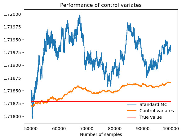
Figure 2. Performance of control variates compared with Monte Carlo when evaluate \( \int_{0}^{1} e^{x} \) .

Table 1. \( \int_{0}^{1} e^{x} \) .

As figure 2 and table 1 show, the performance of control variates is much better than Monte Carlo with an empirical variance reduction of about 98%.

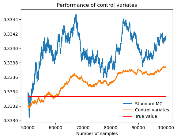
Figure 3. Performance of control variates compared with Monte Carlo when evaluate \( \int_{0}^{1} x^{2} \) .

Table 2. \( \int_{0}^{1} x^{2} \) .

As figure 3 and table 2 show, the performance of control variates is much better than Monte Carlo with an empirical variance reduction of about 94%.

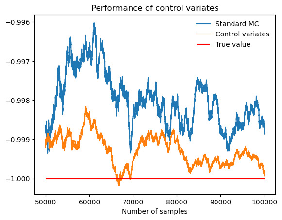
Figure 4. Performance of control variates compared with Monte Carlo when evaluate \( \int_{0}^{1} ln{x} \) .

Table 3. \( \int_{0}^{1} ln{x} \) .

As figure 4 and table 3 show, the performance of control variates is better than Monte Carlo with an empirical variance reduction of about 75%.

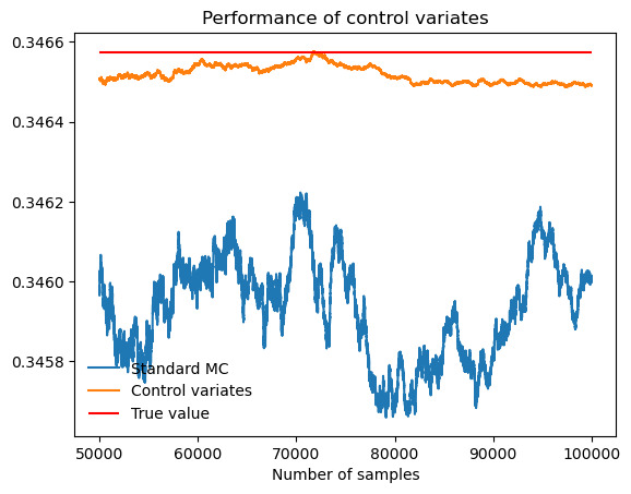
Figure 5. Performance of control variates compared with Monte Carlo when evaluate \( \int_{0}^{\frac{π}{4}} tan{x} \) .

Table 4. \( \int_{0}^{\frac{π}{4}} tan{x} \) .

As figure 5 and table 4 show, the performance of control variates is much better than Monte Carlo with an empirical variance reduction of about 99%.

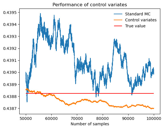
Figure 6. Performance of control variates compared with Monte Carlo when evaluate \( \int_{0}^{1} tan^{-1}{x} \) .

Table 5. \( \int_{0}^{1} tan^{-1}{x} \) .

As figure 6 and table 5 show, the performance of control variates is much better than Monte Carlo with an empirical variance reduction of about 99%. In conclusion, when the functions are monotonic, the effect of variance reduction is usually significant.

4.2 Experiments of other functions

When it comes to double integrals, control variates also work. It is noteworthy that the choosing of variable functions is essential because different variable functions have different correlations and result in different variance reduction. As figure 7 and table 6 show, when the integrand is \( e^{x}*e^{y} \) , there is no remarkable difference between the results of the two variable functions.

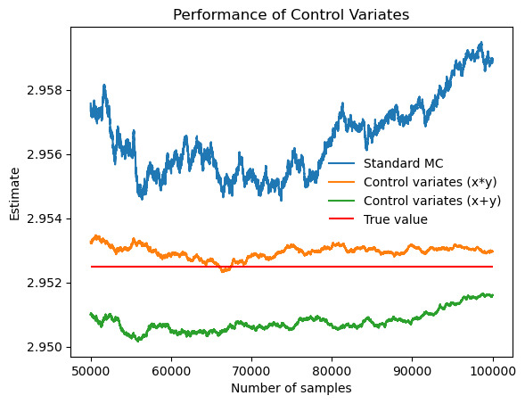
Figure 7. Performance of control variates (x*y) compared with control variates (x+y) and Monte Carlo when evaluate \( \iint_{0}^{1} e^{x}*e^{y} \) .

Table 6. \( \iint_{0}^{1} e^{x}*e^{y} \) .

However, when the integrand is \( e^{xy} \) , as figure 8 and table 7 show, it is obvious that x*y is a better option than x+y when selected variable functions, because in this case where x and y are both between 0 and 1, x*y is smaller than x+y.

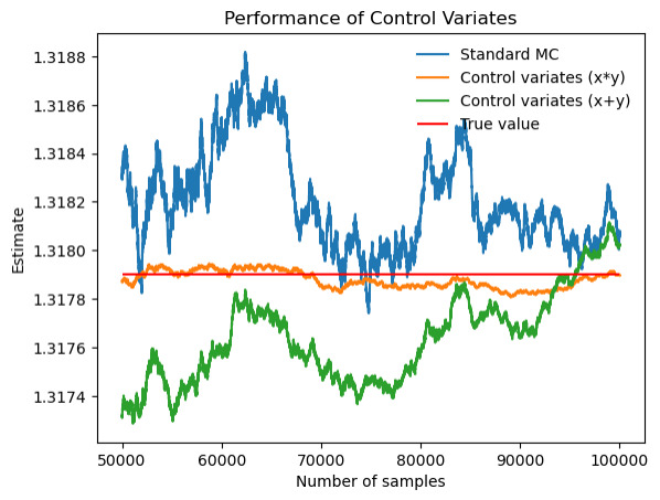
Figure 8. Performance of control variates (x*y) compared with control variates (x+y) and Monte Carlo when evaluate \( \iint_{0}^{1} e^{xy} \) .

Table 7. \( \iint_{0}^{1} e^{xy} \) .

Speaking of functions with infinite intervals, as figure 9 and table 8 show, control variates don't perform well, with only 0.119708 in variance reduction.

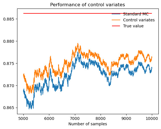
Figure 9. Performance of control variates compared with Monte Carlo when evaluate \( \int_{0}^{∞} e^{-x^{2}} \) .

Table 8. \( \int_{0}^{∞} e^{-x^{2}} \) .

4.3 Splitting method

The functions discussed above are all monotonic functions. Let's discuss functions that are not monotonic. If control variates are used directly, their performance is terrible, which act the same as standard Monte Carlo. But if the function is split into two parts, which are respectively monotonic, and then sum them up, the performance of control variates will improve a lot. This innovative method is called splitting method, and the performance of this new method is called control variates+.

For example, let’s evaluate \( \int_{0}^{1} (x-\frac{1}{2})^{2} \) .

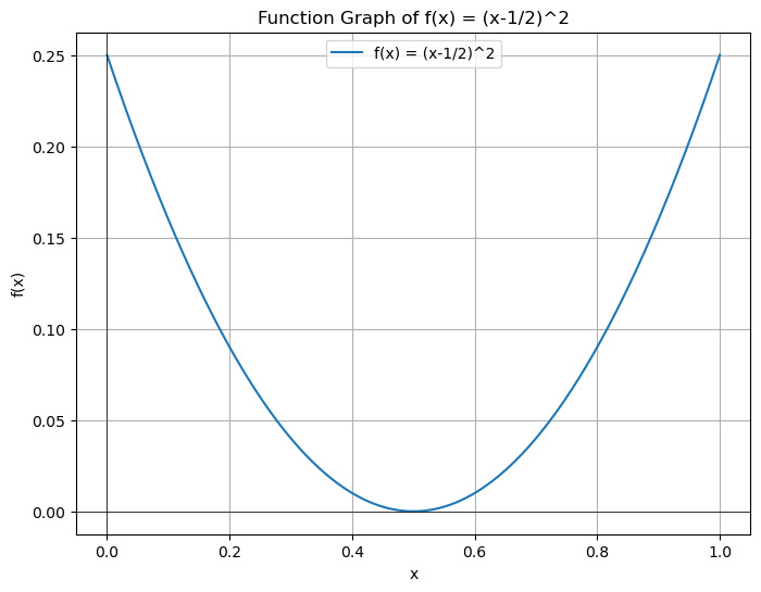
Figure 10. Function graph of \( (x-\frac{1}{2})^{2} \)

Figure 10 shows the function graph of \( (x-\frac{1}{2})^{2} \) .

First, let's directly evaluate \( \int_{0}^{1} (x-\frac{1}{2})^{2} \) .

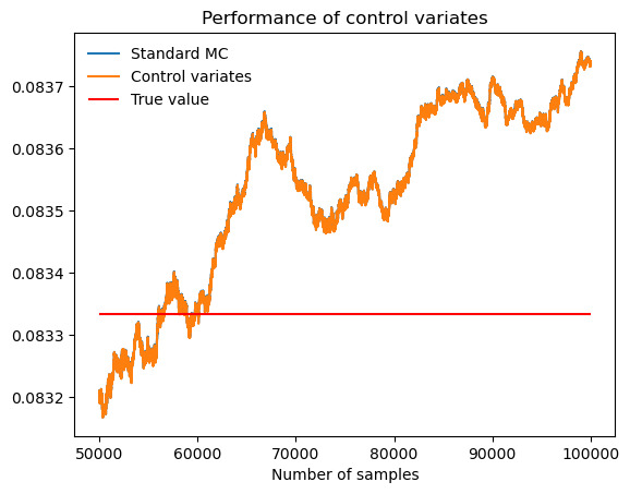
Figure 11. Performance of control variates compared with Monte Carlo when evaluate \( \int_{0}^{1} (x-\frac{1}{2})^{2} \) .

Table 9. \( \int_{0}^{1} (x-\frac{1}{2})^{2} \) .

As figure 11 and table 9 show, control variates and standard MC almost overlap and the variance reduction is only 0. 000044, which means in this case, control variates are nearly useless. Then, let's split the integration interval into two monotonic subintervals and estimate independently in each subinterval.

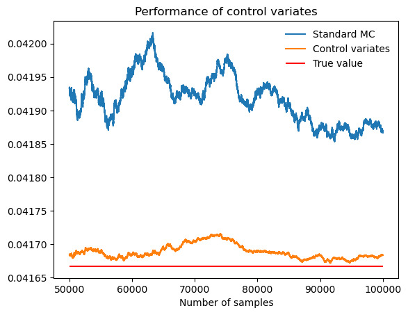
Figure 12. Performance of control variates compared with Monte Carlo when evaluate \( \int_{0}^{\frac{1}{2}} (x-\frac{1}{2})^{2} \) .

Table 10. \( \int_{0}^{\frac{1}{2}} (x-\frac{1}{2})^{2} \) .

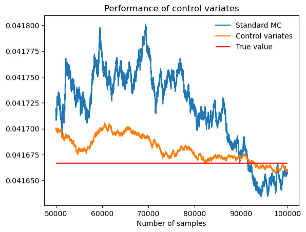
Figure 13. Performance of control variates compared with Monte Carlo when evaluate \( \int_{\frac{1}{2}}^{1} (x-\frac{1}{2})^{2} \) .

Table 11. \( \int_{\frac{1}{2}}^{1} (x-\frac{1}{2})^{2} \) .

As figure 12,13 and table 10,11 show, both the two monotonic subintervals perform well.

After that, let's sum the two results up and obtain the final integral estimate.

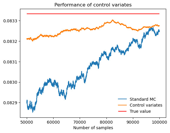
Figure 14. Performance of control variates compared with Monte Carlo when evaluate \( \int_{0}^{\frac{1}{2}} (x-\frac{1}{2})^{2}+\int_{\frac{1}{2}}^{1} (x-\frac{1}{2})^{2} \) .

Table 12. \( \int_{0}^{\frac{1}{2}} (x-\frac{1}{2})^{2}+\int_{\frac{1}{2}}^{1} (x-\frac{1}{2})^{2} \) .

As figure 14 and table 12 show, the final integral estimate performs well. Finally, let's compare the results of control variates with and without splitting method.

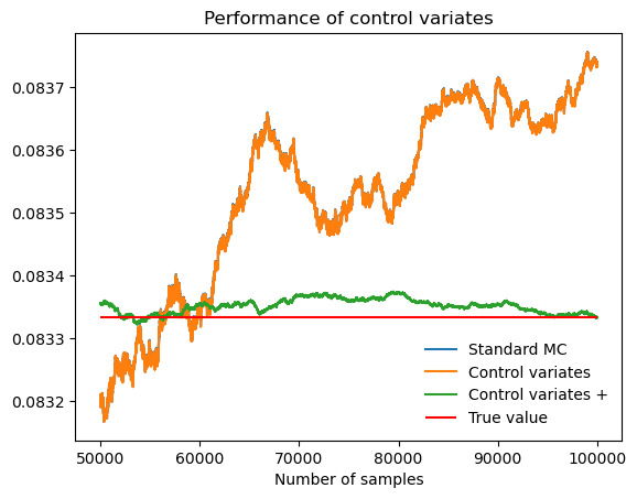
Figure 15. Performance of control variates+ compared with control variates and Monte Carlo when evaluate \( \int_{0}^{1} (x-\frac{1}{2})^{2} \) .

As figure 15 shows, it is evident that control variates+ have a much better performance than control variates. Likewise, as figure 16 shows, integrals like \( \int_{0}^{π} sin{x} \) can also be estimated by splitting method, solving the problem that control variates are useless to estimate integrals with turning points.

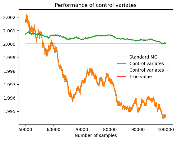
Figure 16. Performance of control variates+ compared with control variates and Monte Carlo when evaluate \( \int_{0}^{π} sin{x} \) .

5 Conclusion

This paper proposes a new numerical integration strategy, which splits the integration interval into several monotonic subintervals and estimate the control variables independently in each subinterval and then the results of each segment can be summed up to obtain the final integral estimate. Such methods minimize the variance inherent in Monte Carlo simulations and improve the accuracy and efficiency of numerical integral estimates. Although the splitting method can solve the problem of estimating the integrals of non-monotonic functions, some oscillating functions, like \( sin{x} \) and \( cos{x,} \) have too many turning points to split, which requires a lot of splitting. And if the splitting method is not used, the direct control variates is almost useless. Therefore, when encountering a function with too many oscillations, variance reduction in Monte Carlo may not help so much.

Acknowledgement

All authors contributed equally to this work and should be considered co-first authors.

References

[1]. Maanane, Y., Roger, M., Delmas, A., Galtier, M., & André, F. (2020). Symbolic Monte Carlo method applied to the identification of radiative properties of a heterogeneous material. Journal of Quantitative Spectroscopy and Radiative Transfer, 249, 107019.
[2]. Zhou, A., Huang, X., Li, N., Jiang, P., & Wang, W. (2020). A Monte Carlo approach to estimate the stability of soil–rock slopes considering the non-uniformity of materials. Symmetry, 12(4), 590.
[3]. Wicaksono, F. D., Arshad, Y. B., & Sihombing, H. (2020). Norm-dist Monte-Carlo integrative method for the improvement of fuzzy analytic hierarchy process. Heliyon, 6(4).
[4]. Sangwongwanich, A., & Blaabjerg, F. (2020). Monte Carlo simulation with incremental damage for reliability assessment of power electronics. IEEE Transactions on Power Electronics, 36(7), 7366-7371.
[5]. Mongwe, W. T., Mbuvha, R., & Marwala, T. (2021). Antithetic magnetic and shadow Hamiltonian Monte Carlo. IEEE Access, 9, 49857-49867.
[6]. Sarrut, D., Baudier, T., Borys, D., Etxebeste, A., Fuchs, H., Gajewski, J., ... & Maigne, L. (2022). The OpenGATE ecosystem for Monte Carlo simulation in medical physics. Physics in Medicine & Biology, 67(18), 184001.
[7]. Song, C., & Kawai, R. (2023). Monte Carlo and variance reduction methods for structural reliability analysis: A comprehensive review. Probabilistic Engineering Mechanics, 73, 103479.
[8]. Yelleni, S. H., Kumari, D., & Srijith, P. K. (2024). Monte Carlo DropBlock for modeling uncertainty in object detection. Pattern Recognition, 146, 110003.
[9]. Mazzola, G. (2024). Quantum computing for chemistry and physics applications from a Monte Carlo perspective. The Journal of Chemical Physics, 160(1).
[10]. Glasserman, P. (2003). Monte Carlo Methods in Financial Engineering. Springer.
Cite this article
Yang,Y.;Zhou,J.;Chen,X. (2024). Variance reduction in Monte Carlo for Integrals. Theoretical and Natural Science,53,203-215.
Data availability
The datasets used and/or analyzed during the current study will be available from the authors upon reasonable request.
Disclaimer/Publisher's Note
The statements, opinions and data contained in all publications are solely those of the individual author(s) and contributor(s) and not of EWA Publishing and/or the editor(s). EWA Publishing and/or the editor(s) disclaim responsibility for any injury to people or property resulting from any ideas, methods, instructions or products referred to in the content.
About volume
Volume title: Proceedings of the 2nd International Conference on Applied Physics and Mathematical Modeling
© 2024 by the author(s). Licensee EWA Publishing, Oxford, UK. This article is an open access article distributed under the terms and
conditions of the Creative Commons Attribution (CC BY) license. Authors who
publish this series agree to the following terms:
1. Authors retain copyright and grant the series right of first publication with the work simultaneously licensed under a Creative Commons
Attribution License that allows others to share the work with an acknowledgment of the work's authorship and initial publication in this
series.
2. Authors are able to enter into separate, additional contractual arrangements for the non-exclusive distribution of the series's published
version of the work (e.g., post it to an institutional repository or publish it in a book), with an acknowledgment of its initial
publication in this series.
3. Authors are permitted and encouraged to post their work online (e.g., in institutional repositories or on their website) prior to and
during the submission process, as it can lead to productive exchanges, as well as earlier and greater citation of published work (See
Open access policy for details).