1. Introduction

Inspired from the Kaggle competition “WSDM – KKBox’s Music Recommendation Challenge” [9], it is meaningful and necessary to build a better music recommender system for a music streaming service (i.e., KKBox, Spotify) as the precise recommendation could provide better user experience [1] .

We will use the dataset from KKBox which includes the information about the first observable listening event for each unique user-song pair within a specific time duration accompanied by the information of users and songs. The aim is to predict whether the song will be recurring listened to by the user within one month after the user’s first listening for a given user-song pair. [9]

The prediction will have 2 possible results, there is a recurring listening event or not, that can be seen as classify the user-song pairs into two classes. Therefore, the problem can be transferred to a classification problem.

In this study, we aim to apply different models to predict the habits of users and compare the performance of built models. We choose three popular classification models for further exploration. K Nearest Neighbors (KNN) is chosen as baseline model, Random Forest and Light Gradient Boosting Machine (LightGBM) are potentially improved models. The details of the methodology will be stated in Section 3.

Based on our experiments, the LightGBM model has the best performance among the three models. That is also consistent with the existing results in the Kaggle competition. In the Kaggle competition, the LightGBM model was heated discussed and the 1st place solution is also partly based on LightGBM. Therefore, the LightGBM seems to be the ideal model for this kind of problem.

2. Related works

As this is a past Kaggle competition, there are many implementations and discussions on Kaggle. The most popular model used is LightGBM and the 1st place solution is also based on LightGBM [10]. Besides, there are also several implementations based on Random Forest, SVD and XGBoost.

The core of the recommender system is the filtering algorithm, especially collaborative filtering [3]. The most popular collaborative filtering algorithm is the KNN [3]. The recommender system based on KNN is conceptually simple and usually gets good-quality results, but also has the cold start problem and low scalability [3]. Another popular approach is based on SVD which can reduce the dimensionality and increase the scalability [13]. Random Forest could avoid the local optimal solutions by assembling a large number of individual decision trees [2]. With the help of the two novel techniques Gradient-Based One-Side Sampling (GOSS) and Exclusive Feature Bundling (EFB) [7], LightGBM can handle the large size of data and takes lower memory [6].

3. Methodology

We use the dataset from the KKBox’s competition. We are asked to predict the probability if a user will listen to a song repetitively after the first listen event based on the given dataset. To wrack this challenge, we plan to start with data analysis, then preprocess the data, and adapt three models to the data to compare and analyze the performance among them.

3.1. Statistical Data Analysis

In this part, we mainly use numpy, and matplot library to help analyze the original dataset, and visualize the data.

The original dataset is divided into 6 tables: train.csv, test.csv, songs.csv, memebrs.csv, sample_submission.csv, and song_extra_info.csv. Generally, we want to preview the data, check total number of entries, column types for each table. We also want to check if there are any null values, outlier data. This will help us determine the strategy for processing the data.

For train table and test table, we cared about how many entries do we have for each user. Does user appear in both tables? Moreover, since music can be categorized into different genres, we need some plots to help represent the distribution of these data. We are also interested in the top k types of music genres and songs that are repeated frequently by users in train table, which will help us to have a more comprehensive understanding on the original data.

3.2. Data Preparation

The data are in several files so the first step is to aggregate all data into one table. We combined the data based on msno (i.e., id for member) and song_id.

3.2.1. Data Cleaning. Based on the result we got from EDA part, we start to process the dataset. We need to remove some duplicated or useless attributes in the set.

For example, in song.csv, we have a column holds the ISRC code for each song. It is used to identify songs, which does the exactly same thing as song_id. But it is not precise, and multiple songs could share the same ISRC. Therefore, we need to remove it. We also separate the target attribute from the table as this is the target value for the classification. The remaining attributes are shown in table 1.

After that, we need to handle the outlier values. For the attribute bd, which indicates the age of the member, the values such as 100 or 0 or negative values for age are definitely not reasonable. Therefore, we set the valid range of bd as 10 ~ 75. Any value outside this range will change to null value which indicates unknown.

For null values, we want to keep it as an independent category, as the null values in the dataset indicates unknown. We drop rows has more than 50% null values.

As values for all the attributes other than song_length can be seen as categories, we want to change song_length to make it consistent with others to simplify our further steps. As the slight difference in the length of song is not matter, we can divide it with 60000 ms which change the unit from ms to minute and round it to integer. After that, we actually divided it into several categories and make the songs having similar length into the same category.

3.2.2. Data Transformation. As the values for attributes represent different categories. We choose to use OneHotEncoder which converts categorical variables to a numerical representation without an arbitrary ordering to encode the dataset [11]. But that also lead to another problem, the encoded data is a high-dimensional sparse matrix. Therefore, we use TruncatedSVD [12] to do dimensionality reduction.

3.2.3. Split Dataset. As the original dataset doesn't provide target values for test data, it's hard for us to do evaluation on it. Therefore, we use the origin train dataset as our whole dataset, and split it for training-validation and testing. We use 4:1 as the split ratio for training-validation and testing datasets and split randomly.

3.3. Implement Models

Based on the dataset, we pick four relatively basic models as the comparison object in our study. We plan to choose the KNN as our baseline model. In addition, Random Forest and LightGBM from Gradient Boosting Decision Trees (GBDT) algorithms will also be used as potentially improved models.

3.3.1. K Nearest Neighbors. K Nearest Neighbors (KNN) is a simple but powerful method for classification [5]. The main idea of KNN algorithm is when there is a new data point comes, pick k neighborhood data points around it and put it to the majority category among k neighborhood data points. As KNN needs to define the k value, we run different k values on the validation set to make decision.

3.3.2. Random Forest. Random Forest is an ensemble learning method for classification operated by constructing a number of decision trees, each of which considers a random subset of features with a random set of training data points. The salient advantage of a random forest model is that it averages all the decision trees to improve the predictive accuracy and control over-fitting. With the help of scikit-learn package, we initiate the RandomForestClassifier model and fit the model on our training data. After training the model, now the model learns some relationship between features and target, we then make predictions on the test data and compare the results with the existing targets.

3.3.3. LightGBM. LightGBM is a high-performance gradient boosting framework based on decision tree algorithm. It splits the tree leaf wise with the best fit which reduce more loss than level-wise algorithm. [8] It provides more accuracy and has a relatively fast training time. We need to test the parameter value for num_leaves and max_depth to gain a better accuracy.

3.4. Comparison & Evaluation

3.4.1. AUC. For the evaluation, we will use the area under a Receiver operating characteristics (ROC) curve (AUC) as the criterion. The ROC graph is a two-dimensional graph which has the true positives (TP) rate as the Y axis and the false positives (FP) rate as the X axis [4]. Generally, the AUC value of a realistic classifier will be between 0.5 and 1, and the closer to 1 means the result is better [4].

3.4.2. Holdout VS. Cross-Validation. For the training-validation dataset, we want to split it into training and validation datasets. We use two ways to split train and validation datasets for the evaluation: Holdout and Cross-Validation.

For the holdout method, we use 3:1 as the split ratio for training and validation datasets and split randomly.

For the Cross-Validation method, we randomly split the data into k mutually exclusive subsets D₁, D₂, ..., D_k with approximately equal size. At the i^th (i = 1, 2, ..., k) iteration, we use D_i as the validation dataset and others as the training dataset. We choose \( k=5 \) for the Cross-Validation.

4. Empirical Results

This section includes the empirical results for the statistical data analysis, data preprocessing and applying three models discussed in previous section.

4.1. Statistical Data Analysis

We start our data analysis based on some related works on Kaggle. This is an essential part, since our model's predict results are directly related to how well we form and reconstruct the dataset.

4.2. Data Preprocessing

Based on our observations on the raw data and EDA results. We start to construct new train dataset and test dataset.

First, we decide to merge original train & test with songs.csv and members.csv by key column “msno” and “song_id” to obtain more comprehensive datasets. Next, we start to handle missing values by replacing all “NaN” value into 0. For age attribute “bd” since it holds continuous value. We want to divide it into 4 categories: [0], (0,25), [25,50), (50,100] based on our EDA results.

After that, like we mentioned in methodology, we convert categorical variables to a numerical representation. Then, we construct a new attribute “artist_repeat_percentage” by counting the repeat times for each artist. So that we can get rid of “artist_name”, “composer”, “lyricist” these attributes that we can't categorize. Finally, we drop some redundant attributes or attributes that we think don't have enough credibility.

The remaining attributes after data preprocessing is listed in table 1:

Table 1. Remaining attributes.

4.3. KNN

We have tried different k values with the two train-validation methods. And the results are shown in Figure 1 and Figure 2.

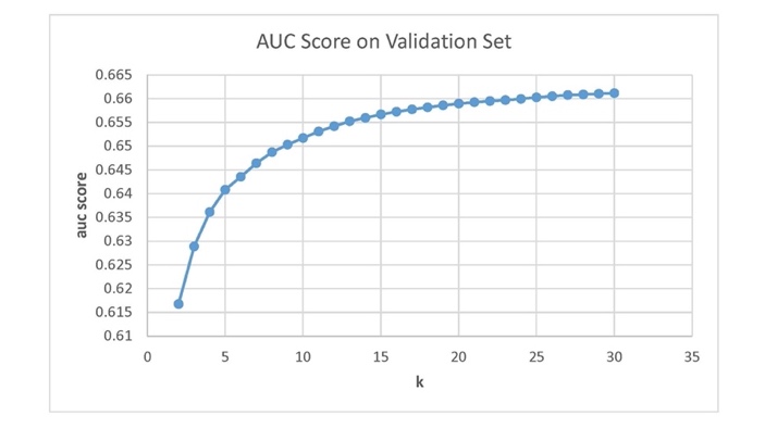
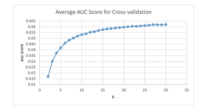
Figure 1 shows the AUC scores using the holdout method for different k values. As the AUC score changed slightly after \( k = 13 \) , we picked up 13 as the k value. AUC score for \( k=13 \) on test set is 0.65456.

Figure 2 shows the average AUC scores using the 5-folds cross-validation method for different k values. As the AUC score changed slightly after \( k = 14 \) , we picked up 14 as the k value. AUC score for \( k=14 \) on test set is 0.65536.

4.4. Random Forest

After tuning the hyperparameters, we pick up the following parameters: \( max depth=20 \) , \( random state=0 \) , \( n estimators=200 \) . Then we evaluate the model and obtain the AUC score on the test set is 0.67416. We also conduct k-fold Cross-validation on this random forest model with 5 folds. For the simplicity to make comparison, mean AUC score of cross validation is given by 0.67269.

4.5. LightGBM

The hyperparameters' values for LightGBM are decided by calling GridSearchCV to help choose the best parameters: \( objective=binary \) , \( eval\_metric=auc \) , \( boosting=gbdt \) , \( learning\_rate=0.1 \) , \( verbose=0 \) , \( num\_leaves={2^{10}} \) , \( max\_depth=50 \) and \( num\_rounds=1000 \) . The prediction results on the test dataset gives AUC score around: 0.71199.

After doing a 5-folds cross validation on training set. It outputs a mean AUC score around: 0.71620. We can see there is a slight improvement by using cross validation comparing to the two train-validation methods.

4.6. Comparison

Table 2 shows the AUC score on testing dataset using holdout method or cross-validation method for the three models, K Nearest Neighbors (KNN), Random Forest (RF) and Light GBM (LGBM).

Table 2. Comparison.

From table 2, the LGBM has the highest AUC score. The AUC scores using holdout method and cross-validation method are similar. The cross-validation scores for KNN and LGBM are a little higher than holdout scores.

5. Conclusions

From the EDA result, we found that both the training set and testing set have a cold start problem. Moreover, we did data preparation based on EDA, including removing attributes, handling outlier and null values, data encoding, dimensionality reduction, and splitting datasets. This part plays an important role when we start training our models. A poor processed dataset is very possible to bring us a model with low prediction accuracy.

After that, we applied three chosen models KNN Random Forest and LightGBM on the processed data on the dataset. According to the evaluation on AUC scores of both holdout method and 5-folds cross-validation method, LightGBM got the highest scores, which means Light GBM performs the best. In addition, Random Forest performs better than the benchmark KNN model.

In the nutshell, LightGBM is an ideal method compared to baseline model KNN and Random Forest method for the Kaggle competition “WSDM - KKBox’s Music Recommendation Challenge”, which complies with existing results in the competition. For the validation part, the cross-validation method can get light better results than the holdout method, but there is no significant improvement. Therefore, the core for improving the recommendation result is still choosing the suitable model and make enough effort on feature engineering. The limitation of the study is that there's still a lot of room for feature engineering and there exist other potentially advanced methods which may also be conducted to make comparisons.

References

[1]. Ananthram, Priya “EDA of music recommendation system” https://www.kaggle.com/ priyaananthram/eda-of-music-recommendation-system
[2]. Belgiu, Mariana, and Lucian Drăguţ.‘‘Random forest in remote sensing: A review of applications and future directions.’’ ISPRS journal of photogrammetry and remote sensing 114 (2016): 24-31.
[3]. Bobadilla, Jesús, et al. “Recommender systems survey.” Knowledge-based systems 46 (2013): 109-132.
[4]. Fawcett, Tom. “An introduction to ROC analysis.” Pattern recognition letters 27.8 (2006): 861-874.
[5]. Guo, Gongde, et al. “KNN model-based approach in classification.” OTM Confederated International Conferences “On the Move to Meaningful Internet Systems”. Springer, Berlin, Heidelberg, 2003.
[6]. Jiang, Jiawei, et al. “Dimboost: Boosting gradient boosting decision tree to higher dimensions.” Proceedings of the 2018 International Conference on Management of Data. 2018.
[7]. Ke, Guolin, et al. “Lightgbm: A highly efficient gradient boosting decision tree.” Advances in neural information processing systems 30 (2017): 3146-3154.
[8]. Khandelwal, Pranjal. “Which algorithm takes the crown: Light GBM vs XGBOOST?” https://www.analyticsvidhya.com/blog/2017/06/which-algorithm-takes-the-crown-light-gbm-vs-xgboost/
[9]. KKBOX. “WSDM - KKBox's Music Recommendation Challenge” https://www. kaggle .com/c/kkbox-music-recommendation-challengef
[10]. lystdo. “A brief introduction to the 1st place solution” https://www.kaggle.com/c/kkbox-music-recommendation-challenge/discussion/45942
[11]. Pedregosa et al. “OneHotEncoder” https://scikit-learn.org/stable/modules/generated/sklearn. preprocessing.OneHotEncoder.html
[12]. Pedregosa et al. “TruncatedSVD” https://scikit-learn.org/stable/modules/generated/sklearn. decomposition.TruncatedSVD.html
[13]. Vozalis, Manolis G., and Konstantinos G. Margaritis. “Using SVD and demographic data for the enhancement of generalized collaborative filtering.” Information Sciences 177.15 (2007): 3017-3037.
Cite this article
Cheng,X.;Liu,K.;Hu,X.;Liu,T.;Che,C.;Zhu,C. (2024). Comparative Analysis of Machine Learning Models for Music Recommendation. Theoretical and Natural Science,53,249-254.
Data availability
The datasets used and/or analyzed during the current study will be available from the authors upon reasonable request.
Disclaimer/Publisher's Note
The statements, opinions and data contained in all publications are solely those of the individual author(s) and contributor(s) and not of EWA Publishing and/or the editor(s). EWA Publishing and/or the editor(s) disclaim responsibility for any injury to people or property resulting from any ideas, methods, instructions or products referred to in the content.
About volume
Volume title: Proceedings of the 2nd International Conference on Applied Physics and Mathematical Modeling
© 2024 by the author(s). Licensee EWA Publishing, Oxford, UK. This article is an open access article distributed under the terms and
conditions of the Creative Commons Attribution (CC BY) license. Authors who
publish this series agree to the following terms:
1. Authors retain copyright and grant the series right of first publication with the work simultaneously licensed under a Creative Commons
Attribution License that allows others to share the work with an acknowledgment of the work's authorship and initial publication in this
series.
2. Authors are able to enter into separate, additional contractual arrangements for the non-exclusive distribution of the series's published
version of the work (e.g., post it to an institutional repository or publish it in a book), with an acknowledgment of its initial
publication in this series.
3. Authors are permitted and encouraged to post their work online (e.g., in institutional repositories or on their website) prior to and
during the submission process, as it can lead to productive exchanges, as well as earlier and greater citation of published work (See
Open access policy for details).