1. Introduction

The housing market is critical to the U.S. economic system. It influences economic stability and reflects economic growth and individuals' well-being. Changes in housing prices can directly reflect and affect economic shifts and personal well-being. Understanding how housing prices change can be valuable for making investment decisions and gaining insights into broader economic and social trends. Therefore, accurate predictions of future housing prices are highly desirable.

In recent years, an increasing Texas Housing market has drawn much attention from investors and researchers. Mikulic pointed out in his study that increasing immigration and tourism have caused the housing market to grow in Texas, even during the Pandemic period [1]. Some other factors, such as labor, the stock, and the mortgage market, have shown influence over the housing market through Antonakakis’ research [2]. Specifically, Hattapoglu and Hoxha pointed out that the tremendous economic growth of Texas in the past decade caused Texas housing prices to be in a growing trend [3]. In addition, Jiao and his team have provided evidence that the relocation of Tesla’s Gigafactory back in 2020 also had a positive effect on Austin’s housing market [4]. With those influential factors and sudden changes in Texas in the past few years make it a great example for analyzing how different they correlate with each other and how they affect housing prices.

Researchers often experiment with different models and methods to produce accurate predictions. Regarding housing prices, predicting with different correlated factors is a conventional method. Teoh used multinomial logistics regression (MLR) and SHapley Additive ExPlanations (SHAP) to analyze the changes in Melbourne and Ames’s housing prices, which those models are effective when evaluating the likelihood ratio of each variable towards a skewed housing price data set [5]. In Zhang’s research, a study of Boston housing prices using the Multilinear Regression model with Spearman Correlation Coefficient considering numerous possible relative factors, including environmental variables and transportation availability, successfully predicts the result to some extent [6]. While those models have shown successful predictions to different degrees, another model that has often been used in forecasting time series and is strongly correlated with other factors is the Vector AutoRegression (VAR) model. Canöz and Kalkavan utilized the Bayesian time-varying VAR(TAR-VAR) model to analyze the macroeconomic variable, demonstrate that inflation and economic growth have a favorable effect on housing prices, and highlight that higher exchange rates attract investment instruments [7]. Another study conducted by Feng, using the VAR to analyze the housing market and monetary policy, suggested a stable long-term relationship between the inflation rate and housing prices [8]. Moreover, as the attention to the field of machine learning began to ramp up in recent years, researchers have discovered new methodologies using machine learning and neural networks to predict housing prices. Guo’s team reported that in research on China’s Housing prices, the innovative machine-learning methodology demonstrated results that outperformed traditional regression models [9]. Similarly, Park and Bae's research also conducted a comparison between different machine learning models with different classifiers and reported the remarkable performance of the Repeated Incremental Pruning to Produce Error Reduction (RIPPER) algorithm in enhancing the predictability of Virginia real estate prices [10].

Overall, housing prices have always been a high-profile topic that has attracted numerous scholars. This research will focus on forecasting future housing prices in Texas, discovering the correlation between influential factors on housing prices using the Autoregression Differencing Moving Average (ARIMA) and VAR models, and providing suggestions for investors and potential buyers.

2. Methodology

2.1. Data sources

In this research, three sets of data are being considered: housing prices, population, and household income. The median housing prices data is obtained from the Texas Real-Estate Research Center, and the later two data sets are accessed through the Federal Reserve Bank of St. Louis. All three data sets are annual data from 1990 to 2022. A total of 33 years of data will allow us to analyze the long-term changes in the Texas housing market.

2.2. Variable selection

The data set of housing prices consists of numerous variables, including average housing prices, median housing prices, sales, dollar volume, etc. In this study, the author chose to use the median price as the data for housing prices. The distribution of housing prices is usually right skewed, using median price as housing price data better reflect typical housing price value. For the same reason, the median household income is chosen to be the household income data.

As shown in Figure 1, Texas housing prices have generally followed a stable upward trend over the past 33 years. From 1990 to 2010, the increase was gradual, but starting in 2011, the trend became more rapid. Beginning in 2020, the increase became even sharper.

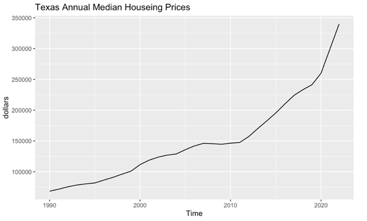
Figure 1: Texas Annual Median Housing Prices.

2.3. Model introduction

Two different time series models are being used in this table. The first one is the ARIMA model. The ARIMA model contains three different parts: Autoregression (AR), Differencing (I), and Moving Average (MA). The AR component is responsible for regressing the lagged(past) value and calculates how the passing value affects the current value. The differencing step removes the seasonality of data by subtracting the current observation from the previous observations and making the time series stationary. The MA part captures the errors of past terms and considers their influence over the current term.

The VAR model is a generalization of the univariate autoregressive model used for forecasting a vector of time series. In the VAR model, all variables are treated symmetrically, meaning they all influence each other equally. An important parameter in the VAR model is variable p, which refers to the number of lags included in a linear combination. The VAR model evaluates the correlation between previous lags and the current value. For instance, a second-order VAR model would use data from the two previous time periods to evaluate how the past two data sets affect the current data. Since the VAR model analyzes and forecasts time series simultaneously, it has been widely used in economic analysis, natural science, and housing prices. This article will use population and household income to build the VAR model with housing prices.

3. Results and discussion

3.1. Space considerations

Both ARIMA and VAR models require stationary data, so the first step is to ensure the stationarity of all data sets. Figure 2, 3 and 4 display the ACF graph of housing prices, population, and household income time series. All three ACF graphs showed similar behavior. A high autocorrelation can be observed in the first few lags, and it quickly diminishes to zero in the following few legs, showing signs of stationarity among these time series. Thus, no further data processing is needed.

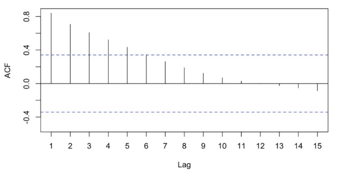
Figure 2: The ACF Plot of Housing Prices

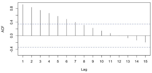
Figure 3: The ACF Plot of Population

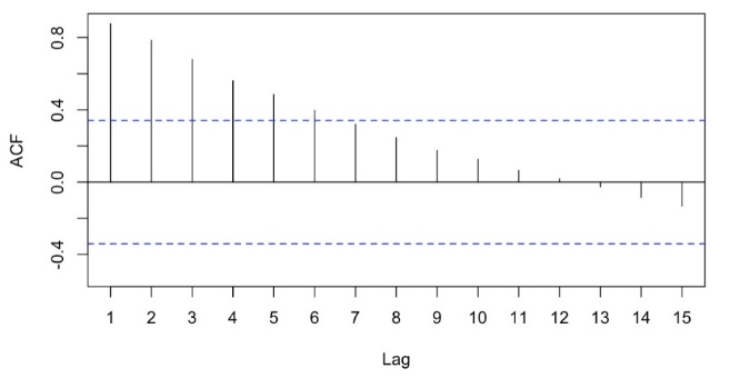
Figure 4: The ACF Plot of Household Income

3.2. Model evaluation

Various aspects and variables can be considered when evaluating the performance of a model. Two conventional ways of evaluating the model are comparing the fitness of the model to the data and the accuracy of the forecast on data that hasn’t been presented to the model. The better-fitted model and better forecast on unseen data would presumably be considered the better model. Therefore, this article uses two variables to evaluate the model performance (Table 1).

The first one is the Akaike Information Criterion (AIC) value, which evaluates the fitness of a model to the data. A lower AIC value indicates better fitness. However, AIC assumes an infinite amount of data, that more data would lead to better accuracy, and that the data set being studied only contains 32 observations. Therefore, instead of using the AIC value, the Akaike Information Criterion correction (AICc) value will be used. The AICc value converts the result of AIC into a large sample size by adding a correction term, allowing smaller sample size data to fulfill the AIC assumption.

The second variable is Mean Absolute Percentage Error (MAPE), which measures the mean absolute error percentage between actual data and forecast data. In order to evaluate how models perform on unseen data, the data set will be split into two parts. The first part will be the training set, which contains data from 1990 to 2017, and the second part will be the testing set, which will be data from 2018 to 2022. The table below presents the results of different models.

Table 1: Evaluation Table

As Table 1 shows, the ARIMA model has the lowest AIC value and the lowest MAPE value, showing a better overall performance. Among all different kinds of VAR models, the VAR model with housing prices and population when p = 5 has the lowest AIC value. However, it also has the highest MAPE value. The model best fits the data but performed poorly when engaging with unseen data, which indicates signs of overfitting. The VAR model with housing prices and household income (p = 3) has a relatively lower MAPE value and a relatively median AIC value. Therefore, the article believes that it has the best performance among VAR models. The next step is to use the ARIMA model and VAR model with household income and housing prices (p = 3) to generate forecasts on future housing prices.

3.3. Forecasting

Figure 5 and 6 present the results of ARIMA and VAR forecasts for the next decade.

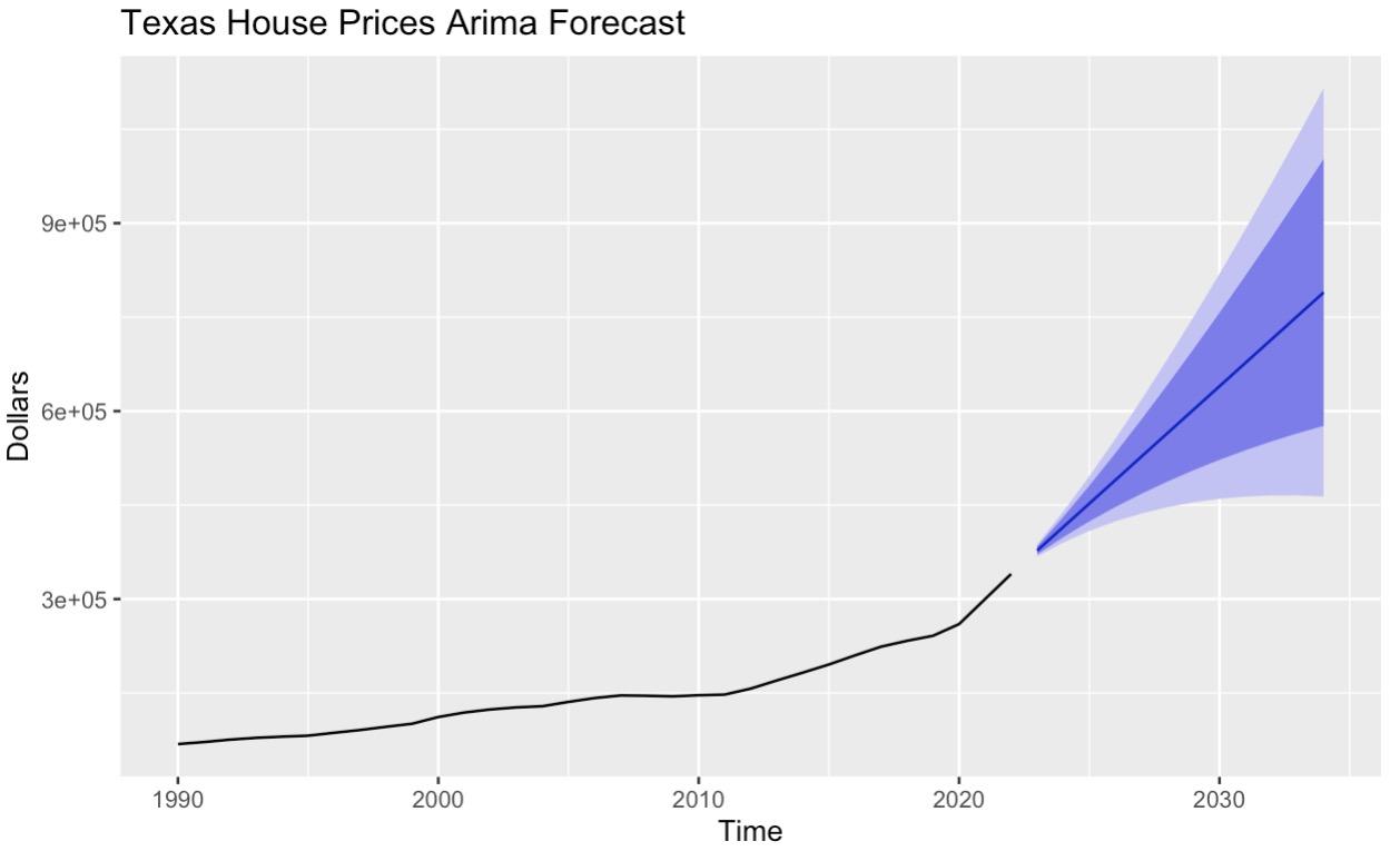
Figure 5: ARIMA(0,2,1) Forecast on Texas Housing Prices

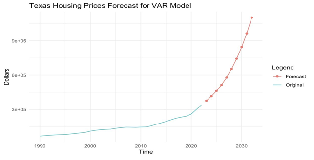
Figure 6: VAR Forecast on Texas Housing Prices

Both models provide a forecast showing a continuously increasing trend in housing prices. The ARIMA model possesses a relatively more gradual increasing trend, and the VAR model is increasing more rapidly.

3.4. Check residuals

The last step is to check the reliability of the model and ensure it resembles white noise and is suited for forecasting. Figure 7 shows the residual plot of the ARIMA model. As the ACF plot shows, the autocorrelation of all lags is below the dashed line representing the significance level. This indicates that the model resembles white noises, showing evidence for the suitability of forecasting. Table 2 shows the result of the Ljung-Box test for the ARIMA model, and the p-value is significantly bigger than 0.05, further proving the ARIMA model's reliability.

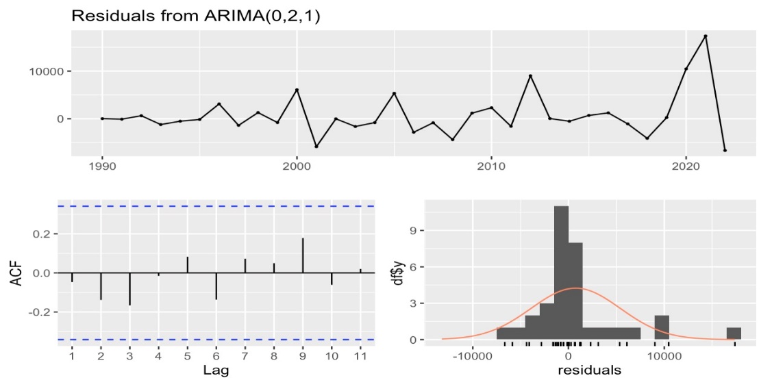
Figure 7: Residuals from the ARIMA Model

Table 2: Ljung-Box Test for ARIMA Model

Table 3: Portmanteau Test for VAR Model

Table 3 shows the result of the Portmanteau Test for the VAR model, and the p-value for the test is 0.5198, which is significantly greater than 0.05, indicating that the model resembles white noise and is suitable for applying forecasts.

3.5. Critical thinking

Both models have shown good performance in regard to model fitness and forecast accuracy. The ARIMA model outperforms the VAR model in both aspects with a slight advantage. Nevertheless, it does not mean that the ARIMA model is always better when considering housing price forecasts.

Table 4: Summary Table of VAR model

Table 4 presents the summary table of the VAR model. The rightmost P-value column provides the p-value for each lag. A p-value smaller than 0.05 indicates a significant statistical influence of the specified lag over the current value. While the price’s lag provides the most significant influence over the current value, the lag 1 of income also showed a significant positive effect over the current value. It’s evident that there is a significant correlation between household income and housing prices. Therefore, it is still reasonable to consider using the VAR model to perform housing price forecasts, even if the accuracy of the VAR model is slightly lower.

4. Conclusion

As both models suggested an increasing trend for Texas housing prices, it is reasonable to recommend investors to invest in Texas real estate property. As the population and income keep increasing, housing prices presumably are anticipated to keep growing for the next decades. However, while rising housing prices favor property investment, they may also put pressure on housing affordability. As prices continue to increase, it will become more challenging for first-time buyers and lower-income households to purchase a living place. This article believes that action and policy from the government are crucial to balance the leverages.

In conclusion, both models have predicted an increasing trend in housing prices for the next decade. By evaluating the model, this article concludes that the ARIMA model has a better performance than the VAR model, with household income as a correlated variable. However, the housing market is a complex and dynamic system that is influenced by numerous factors. Average household income is only one factor that has an inner relationship with housing prices. Many other factors, such as mortgage rate or GDP, may also have a significant correlation with housing prices, and experiments with those variables may have the potential to generate a more accurate prediction.

References

[1]. Mikulić J V, et al. 2021 The effect of tourism activity on housing affordability. Annals of Tourism Research, Elsevier, 90.
[2]. Antonakakis N, Chatziantoniou I and Gabauer D 2021 A regional decomposition of US housing prices and volume: market dynamics and portfolio diversification. Ann Reg Sci, 66, 279-307.
[3]. Hattapoglu M and Hoxha I 2021 Hot and cold seasons in Texas housing markets. International Journal of Housing Markets and Analysis, 14, 317-332.
[4]. Jiao J F, et al. 2023 International Journal of Housing Markets and Analysis. Bingley, 16, 628-641.
[5]. Teoh E Z, Yau W C, Ong T S and Connie T 2023 Explainable housing price prediction with determinant analysis. International Journal of Housing Markets and Analysis, 16(5), 1021-1045.
[6]. Zhang Q 2021 Housing price prediction based on multiple linear regression. Scientific Programming, 7678931.
[7]. Canöz İ and Kalkavan H 2024 Forecasting the dynamics of the Istanbul real estate market with the Bayesian time-varying VAR model regarding housing affordability. Habitat International, 148.
[8]. Feng P 2022 The correlation between monetary policy and housing price change based on a VAR model. Mathematical Problems in Engineering.
[9]. Guo J Q, et al. 2020 Can machine learning algorithms associated with text mining from internet data improve housing price prediction performance? International Journal of Strategic Property Management, 24(5), 300-312.
[10]. Park B and Bae J K 2015 Using machine learning algorithms for housing price prediction: The case of Fairfax County, Virginia housing data. Expert Systems With Applications, 42(6), 2928-2934.
Cite this article
Wu,Z. (2025). Time Series Forecasting of Texas Housing Prices: A Comparison Between the ARIMA and VAR Models. Theoretical and Natural Science,80,20-27.
Data availability
The datasets used and/or analyzed during the current study will be available from the authors upon reasonable request.
Disclaimer/Publisher's Note
The statements, opinions and data contained in all publications are solely those of the individual author(s) and contributor(s) and not of EWA Publishing and/or the editor(s). EWA Publishing and/or the editor(s) disclaim responsibility for any injury to people or property resulting from any ideas, methods, instructions or products referred to in the content.
About volume
Volume title: Proceedings of the 4th International Conference on Computing Innovation and Applied Physics
© 2024 by the author(s). Licensee EWA Publishing, Oxford, UK. This article is an open access article distributed under the terms and
conditions of the Creative Commons Attribution (CC BY) license. Authors who
publish this series agree to the following terms:
1. Authors retain copyright and grant the series right of first publication with the work simultaneously licensed under a Creative Commons
Attribution License that allows others to share the work with an acknowledgment of the work's authorship and initial publication in this
series.
2. Authors are able to enter into separate, additional contractual arrangements for the non-exclusive distribution of the series's published
version of the work (e.g., post it to an institutional repository or publish it in a book), with an acknowledgment of its initial
publication in this series.
3. Authors are permitted and encouraged to post their work online (e.g., in institutional repositories or on their website) prior to and
during the submission process, as it can lead to productive exchanges, as well as earlier and greater citation of published work (See
Open access policy for details).