1. Introduction

As a robotics enthusiast, I have dedicated extensive time and effort to creating various robotic structures, circuits, and programs, resulting in impressively functional robots. However, the deeper I delve into this field, the more I recognize the risks associated with rigid robotic structures. My experience of being accidentally hurt by my robots and incidents like a chess-playing robot injuring a child's hand have reinforced this concern. These experiences have led me to explore the field of soft robotics.

With their inherent safety for human interactions, soft robots also excel in tasks involving confined spaces and delicate objects. Despite these advantages, current research on soft robots, particularly soft robotic arms, predominantly focuses on tracking the end effector's location to aid in control mechanisms such as forward and inverse kinematics and optimal control. However, this focus often overlooks the development of soft robotic intelligence, which critically depends on the robot's ability to perceive its own form and surroundings.

Currently, the popular deformation control of pneumatic soft robots usually adopts two approaches: open loop control based on the mapping relationship between air pressure [1] and morphology and feedback control based on visual servo [2]. The first one fails when the robot is in contact with items, and the second one relies on the visual servo so it cannot operate under confined circumstances. The works about object perception for soft robots are also popular. For example, Shu et al. embedded strain gauges into a pneumatic soft gripper for the target's size identification [3]. However, the disadvantages caused by the sensor's non-stretchable nature led to the development of stretchable or fluid-based strain sensors [4]. The fluid-based sensors often face the problem of complex structures, which makes them hard to fabricate.

This paper proposes the development of a pneumatic soft robotic grasper and a mathematical model that enables self-shape perception and object-shape perception, thereby enhancing the intelligence of soft robots. A key challenge in this endeavor is the potential inaccuracy caused by changes in air pressure that do not immediately alter the robot's shape when the robot contacts a rigid object. To address this, I propose using a non-intrusive flexible sensor attached to the robot and a corresponding model to improve the accuracy and reliability of the robot's deformation estimation. Using both models, a differential method that estimates the size of the gripping object is proposed.

Several key questions need to be addressed to validate this concept: (1) What material should be used for the sensor, and where should it be located for optimal effectiveness? (2) What theoretical frameworks and formulas can construct a robust and accurate self-shape perception model based on sensor outputs? (3) How can this model be utilized to detect the shapes of objects being gripped? (4) What experimental methods should be employed to investigate and evaluate the research outcomes? Driven by these questions, this paper proposes a new model for soft robots that enhances their perceptual capabilities.

The paper's content is as follows: I explain the main principle behind the self-shape and gripping-object shape perception capabilities and the fabrication process in the second section. Then, in the third section, I cover the mathematical model that outputs the precepted self-shape of the robot from both the sensing signal and the pneumatic pressure. In the fourth section, I showcase the experimentations that evaluate the performance of the robot model, and the conclusion is covered in the sixth section.

2. Methodology

2.1. Principle

A three-segment liquid metal sensor is placed at the bottom of each robotic finger to achieve self-shape and object-shape perception. When actuated by pneumatic pressure, the robotic fingers deform, mainly the axial elongation and bending. Since the resistance of a resistor is positively related to its length, the resistance of the liquid metal sensors would increase as it is elongated with the robotic fingers. Using the resistance change as a signal, a mathematical model develops a mapping between the detected signal and the self-shape perception.

Using the resistance from a simultaneously deforming sensor provides better performance than the traditional pneumatic pressure method. When contacting an object, the robotic fingers' inner pneumatic pressure can continue to increase while the shape of the robotic fingers stays the same. Thus, when a model relies on the detection of pneumatic pressure, the sensing results could be primarily deviated from the actual situation and deformation of the robot. On the other hand, using a sensor that can deform simultaneously with the robotic fingers can accurately capture the deformation of the fingers at any instance, as the deformation of the sensors is precisely the deformation of the fingers. Nevertheless, the project's sensing system employs both methods to reach a more accurate sensing result. Using both sensing systems also enables the robot to sense the instances of contact when seeing an increasing pneumatic pressure with a constant resistance change.

.

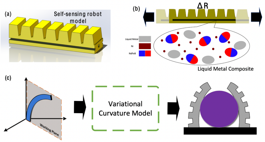
Figure 1: The general principle of the sensing system

The three-segment structure of the sensor realizes the object-shape perception function. The three segments separated one robotic finger into three parts from top to bottom. The three segments will be subjected to different curvatures when gripping objects with different shapes. For example, the three segments would be at similar curvature when gripping a cylinder. In contrast, when gripping a cube, the first and third segments will be subjected to higher curvature than the second. The resistance changes from different segments of the fingers would construct data points that can be used to develop algorithms to estimate the gripping object shape. The experimentation section includes a statistical analysis that can be performed to determine if the data are significantly different, and thus validating its ability to percept gripping object shape.

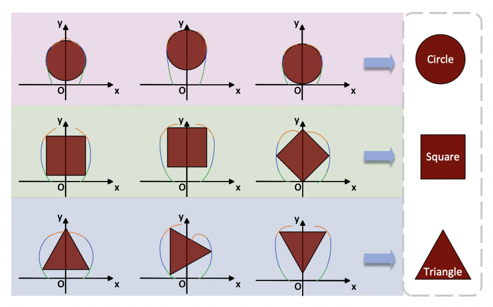
Figure 2: The principle of object-shape sensing

2.2. Design

The structure of the robotic finger is chosen because it is simple to deform and efficient in gripping objects. The thicker limiting layer in the bottom and the air chambers cause the finger to deform in a fixed direction. In this case, the mathematical model would be simplified to two-dimensional since the range of movement is a working plane rather than a working space.

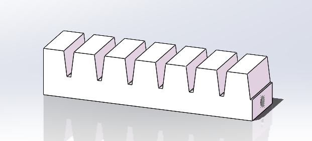
Figure 3: The preliminary design of the robotic finger structure.

Since the project does not emphasize structural design, the kestrel model is a ready-made CAD model from the “MakeSoftRobot” project [5]. The structure features a three-finger robotic structure that includes the mold for the silicone fingers and the holder of the fingers. To cater to the engineering goal, the bottom layer of the finger was altered to be thinner from the mold. This would ease the effort to integrate the three-segment sensor on the bottom of the fingers.

Due to the high conductivity of liquid metal, its resistance is comparatively small and thus its resistance changes in a smaller scale. To resolve this problem, a signal amplification circuit is designed to enlarge the resistance change signal when it is communicating to the computer. To reach this effect, the traditional ratio amplification circuit structure was used to enlarge the received signal before it was communicated to the Arduino chip.

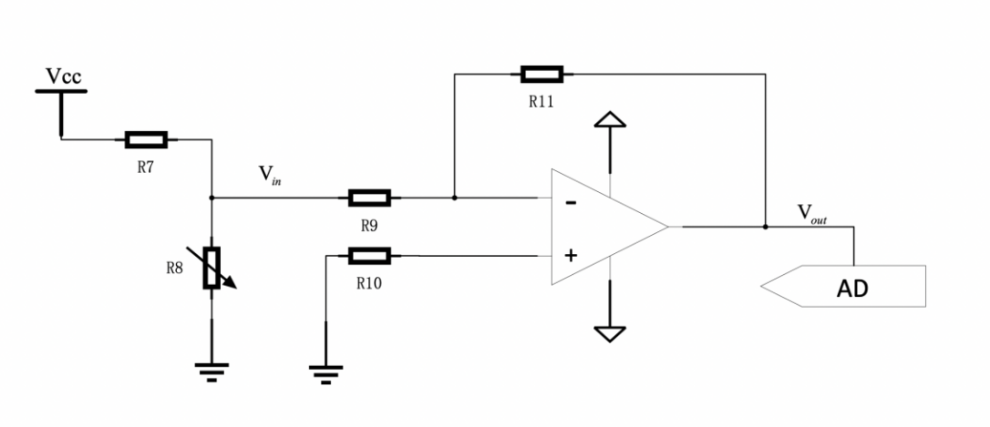
Figure 4: Signal Amplification Circuit

Since each sensor segment requires one ratio amplifier, six amplification circuits with the same structure should be applied to fulfill the needs of the six sensor segments. While signal amplifying is one function of the circuit, the circuit must also communicate the resistance change to the Arduino chip and, thus, to the computer. The signal amplification circuit is then connected to a voltage-dividing circuit. There will be one resistor with fixed resistance connected in series with each of the sensors of the robot fingers. Give this circuit a fixed voltage from the power source and a voltmeter connected for either of the two resistances; the ratio between the voltage of the two resistances can be calculated, which is also the ratio between the resistances. By measuring the voltage of one resistor, the ratio and, thus, the resistance change for the sensor can be calculated. The measured resistance will then be amplified.

A GUI program was developed in Python to visualize the result from the mathematical model. The program receives the sensing signal in digital form via the serial port from an Arduino chip. The program then converts the digital signal to the original resistance value, an inverse transformation of the resistance change to a numerical value by the Arduino chip. Then, with the converted resistance value as the input, the program runs the mathematical model, which produces a curvature value that defines the shape of the robotic fingers. Matplotlib will then visualize the result.

2.3. Sensing Material

The material chosen for the sensor is Ga-In-Sn alloy in the formula of \( {Ga_{68.5}}{In_{21.5}}{Sn_{10}} \) with a melting point of -19°C. The low freezing point of the material will enable the sensor to be capable under situations with temperature lower than 0°C. However, using raw Ga-In-Sn alloy would make the fabrication process hard due to the high surface tension of the liquid metal material. The high surface tension will cause the material to repel the sensor's silicone substrate. Thus, it is decided to find a process that will ease fabrication.

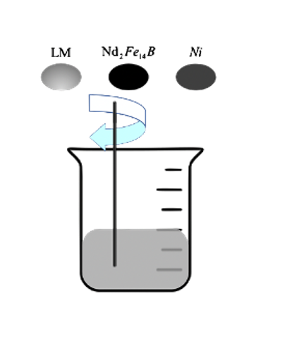
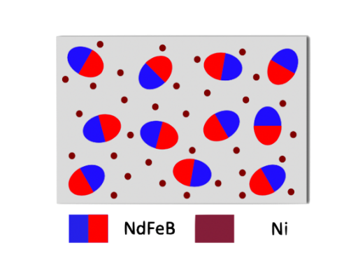
Figure 5: The Liquid metal compound

It is found that the addition of neodymium iron boron ( \( {Nd_{2}}{Fe_{14}}B \) ) and nickel ( \( Ni \) ) particles into the liquid metal would effectively reduce the surface tension of the liquid metal material and make it unsensitive to both tension and pressure [6]. The porous structure formed by the \( NdFeB \) and \( Ni \) particles can store the liquid metal materials and thus lead to the reduced surface tension. Also, as a soft magnetic medium with high permeability, submicron or nanoscale nickel microspheres can increase the magnetic force between magnetized NdFeB particles. With this alteration, the liquid metal and magnetic particle composite will repel less to the silicone substrate and the removal of extra material to the substrate will now not affect the material already filled into the substrate. Thus, this alteration highly eased the fabrication process.

The Ga-Ln-Sn/Ni/NdFeB composite is prepared by mechanical stirring. Ga–In–Sn, Ni, and NdFeB are placed in a container at a mass ratio of 5:2:3 and stirred for 30 min by the author. Table 1 provides the material parameters of the material:

Table 1: Material paramters

2.4. Fabrication

The fabrication process starts with the fabrication of the robotic fingers. From the CAD model which provides a mold that can be used to cast the robotic finger, the fingers are created using the Ecoflex-0050 silicone. The mold can be separated into three parts including the main mold, the lid, and the air chamber separator as shown in figure 6.

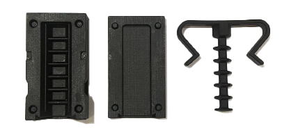
Figure 6: The mold for the robotic fingers.

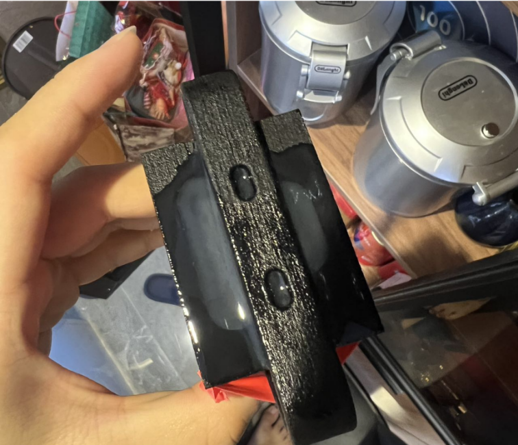
Figure 7: Picture of casting the robotic finger.

Due to the lack of vacuum equipment to eliminate the bubbles within the liquid silicone, I chose to store it under cold temperatures, which will increase the “flowability” of the silicone and accelerate the speed at which bubbles get out. However, this method still cannot eliminate some small bubbles deep down in the silicone, and thus, the robotic fingers are not perfectly free of bubbles. However, the presence of the bubbles does not affect the normal performance of the fingers.

The sensor material is simply created by mixing purchased liquid metal material with the nanomagnetic particles. A mold is needed to fabricate the three-segment sensor to put the liquid metal material into a specific structure. A CAD mold is created to cast a silicone mold that can hold the sensor material, as shown in Figure 8. After the silicone mold is filled with the sensor material, another layer of silicone seals the sensor. Later, these sensors, with liquid metal held within a silicone mold, are stuck to each robot's finger's bottom by some liquid form silicone, as shown in Figure 9.

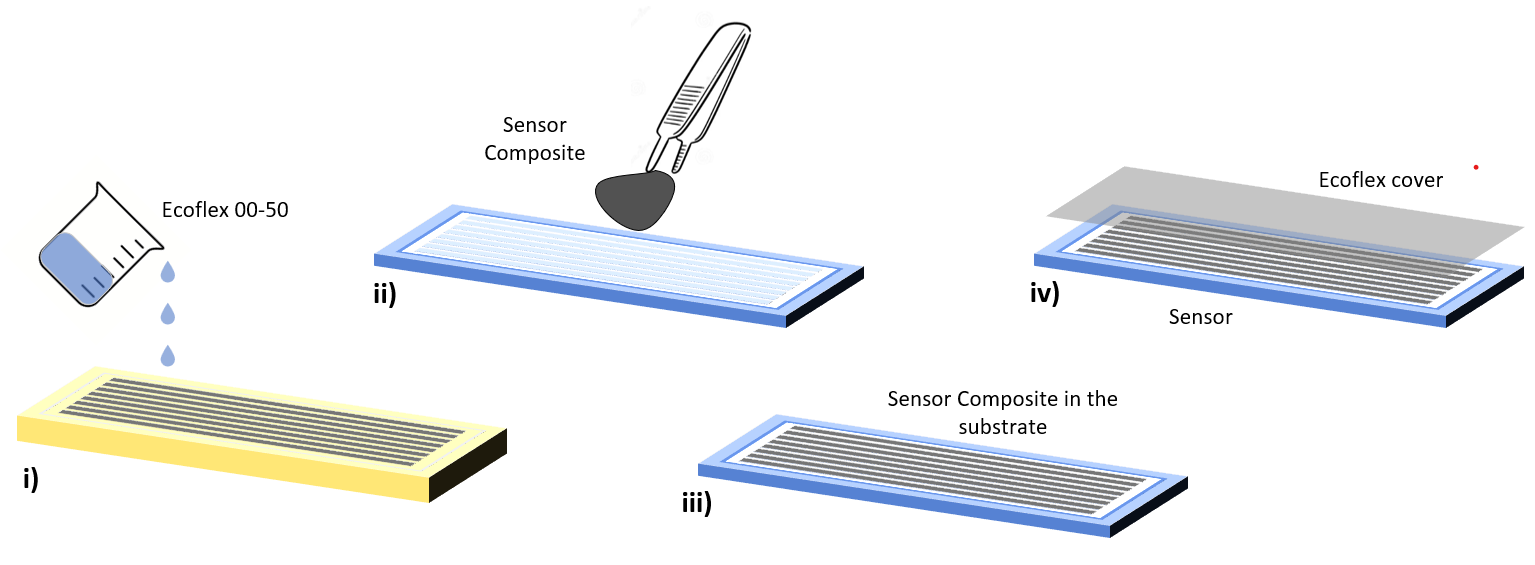
Figure 8: Mold for the sensor and its holder.

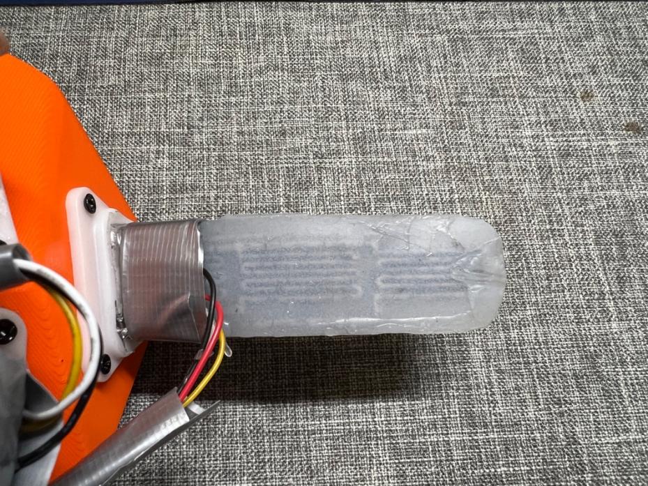
Figure 9: The integrated sensor.

The next step is to create the signal amplification circuit for the sensor. Since there are six sensors, I purchased a six-way ratio amplifier. Following the previously designed circuit structure, I attached the sensor as the variable resistor and all the circuit modules to the structure of the robotic grasper, as shown in Figure 10.

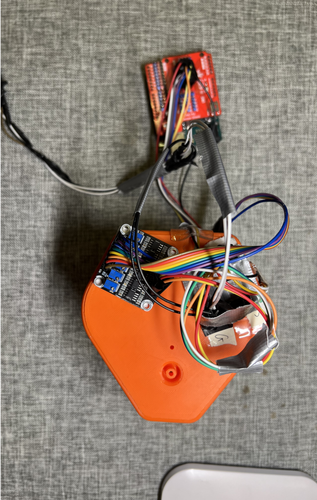
Figure 10: The amplification and voltage-dividing circuit on the grasper.

An actuator is needed to drive the robotic grasper. It supplies pneumatic pressure for the robot and includes the Arduino chip that communicates the received data from the sensor to the computer via serial port.

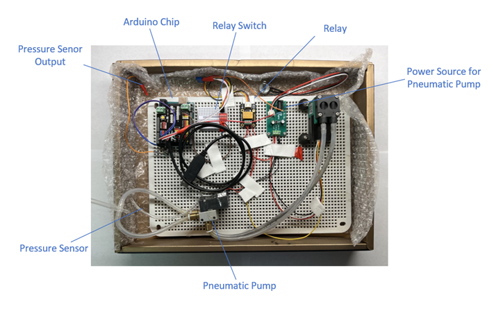
Figure 11: The actuator with labeled parts.

Starting with the actuating module mainly consists of the pneumatic pump, the power supply, the relay and its switch, and the tube that connects the pump to the robot. The power supply provides a 5-volt voltage to the pneumatic pump. The relay and its switch control the mode of the pneumatic pump – the binary switch decides whether the pump sucks air in or pumps air out. The pump is then connected to the air tube, which is also connected to the robotic grasper. On the other hand, the Arduino chip is connected to the signal amplification circuit and to a serial port USB. In this way, the signal from the sensor can be communicated to the computer. The Arduino chip converts the analog electrical signal from 0 to 5 volts to the digital signal from 0 to 1023. A GUI model is then developed to use the digital data to visualize the modeling result.

3. Mathematical Model

3.1. Geometric model and initial assumptions

To develop a mathematical model that estimates the deformation of the robotic finger, an initial geometric model that describes the position and shape of the robotic fingers by its basic physical quantities must be created.

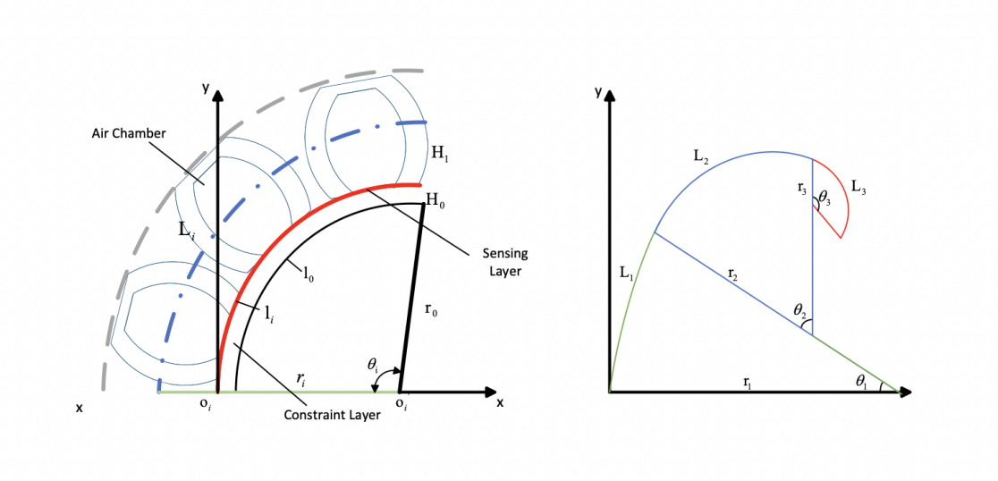
Figure 12: The initial geometric model

As shown in Figure 12, the established geometric model took on a variable curvature assumption, which assumes that the shape of the finger can be represented by its centerline and that every part of the finger experiences elongation under pneumatic pressure. The significance of a variational curvature assumption instead of a constant curvature assumption is that it considers the flexible constraint layer of the robotic finger. Instead of having a fully rigid constraint layer, the robotic finger's bending deformation relies on the different rigidities of the upper and bottom layers. The deformation will possess a variable curvature due to the increasing pneumatic pressure that continuously enlarges the difference in curvature of the two layers, ultimately changing the curvature of the entire structure.

A multi-chamber bending deformation sensing unit is given in Fig.4a. Here, a sensing unit is composed of three air chambers, a constrained layer, and a sensing layer (including a single liquid metal sensor). We define L₀, l_i, and L_i as the bottom arc length of the constraint layer, the sensing layer, and the axial centerline, respectively. Notice due to the variable curvature assumption, L₀ is not a fixed quantity, and it is also assumed that the bottom-constrained layer elongates to provide the basis for the validity of the sensor. H₀ is the thickness of the constraint layer, and H₁ is the thickness of the sensing layer from the centerline. r₀ and r_i are the radius corresponding to arcs L₀ and L_i, respectively, and θ_i is the bending angle. From the figure, we can obtain the following geometric relationships:

\( \begin{cases} \begin{array}{c} {r_{i}}={H_{1}}+{H_{0}}+{r_{0}} \\ {l_{0}}={θ_{i}}\cdot {r_{0}} \\ \begin{matrix}{l_{i}}={θ_{i}}\cdot ({H_{0}}+{r_{0}}) \\ {L_{i}}={θ_{i}}\cdot ({{H_{1}}+H_{0}}+{r_{0}}) \\ \end{matrix} \end{array} \end{cases} \) (1)

Here, it is assumed that the centerline L_i equivalent to the robotic finger and assume the main elongation ratio of the PSA are λ₁^’, λ₂^’ and λ₃^’. According to Eq. (1), the axial elongation of the PSA can be expressed as:

\( λ_{1}^{ \prime }=\frac{{L_{i}}}{{l_{0}}}=\frac{{l_{0}}+{θ_{i}}({H_{1}}+{H_{0}})}{{l_{0}}} \) (2)

3.2. Hyperelastic Model of Silicone

Hyperelastic materials are the materials that have high Poisson ‘s ratio and is assumed to be incompressible. The behavior of this type of material, or the relationship between strain and stress cannot be described by the general Hooke’s law which states a linear relationship between the strain and stress of a material. Hyperelastic models were born to the need of describing the non-linear strain-stress relationship of hyperelastic materials. The material of the robotic finger is silicone, which is hyperelastic.

In this section, we use the Mooney-Rivlin model [7] to describe the deformation of the proposed PSA. The strain energy density function W can be expressed as:

\( W=W({I_{1}}, {I_{2}}, {I_{3}}) \)

\( \begin{cases} \begin{array}{c} {I_{1}}={{λ_{1}}^{2}}+{{λ_{2}}^{2}}+{{λ_{3}}^{2}} \\ {I_{2}}={{λ_{1}}^{2}}{{λ_{2}}^{2}}+{{λ_{2}}^{2}}{{λ_{3}}^{2}}+{{λ_{3}}^{2}}{{λ_{1}}^{2}} \\ {I_{3}}={{λ_{1}}^{2}}{{λ_{2}}^{2}}{{λ_{3}}^{2}} \end{array} \end{cases} \) (4)

\( {λ_{i}}=1+{ε_{i}} \)

where \( {I_{1}} \) , \( {I_{2}} \) , and \( {I_{3}} \) are the first, second, and third invariants of the deformation tensor, respectively. And \( {λ_{i}} \) is the main elongation ratio of the material, and \( {ε_{i}} \) is the main axis strain.

Assuming that the deformation of the silicone material is isotropic and uniform, The strain energy density function can be expressed as an N-order polynomial as the following:

\( W=\sum _{i=1}^{N}\sum _{j=1}^{N}{C_{ij}}{({I_{1}}-3)^{i}}{({I_{2}}-3)^{j}}+\sum _{i=1}^{N}\frac{1}{{D_{i}}}{(J-2)^{2i}} \) (5)

Where \( {C_{ij}} \) is the Rivlin coefficient, \( {D_{i}} \) the incompressibility parameter, and \( J \) the volume change ratio, which is \( {λ_{1}}{λ_{2}}{λ_{3}} \) .

Thus, the second-degree Mooney Rivlin model can be expressed as the following:

\( W={C_{10}}({I_{1}}-3)+{C_{01}}({I_{2}}-3) \) (6)

By the incompressibility characteristic of hyperelastic materials, the volume change ratio \( J=1 \) and thus can be neglected in the stress energy function. By definition, the main axial stress is related with the strain energy by:

\( {σ_{1}}={λ_{1}}\frac{∂W}{∂{λ_{1}}}={λ_{1}}(\frac{∂W}{∂{I_{1}}}\frac{∂{I_{1}}}{∂{λ_{1}}}+\frac{∂W}{∂{I_{2}}}\frac{∂{I_{2}}}{∂{λ_{1}}}) \) (7)

Which is

\( {σ_{1}}=2{C_{10}}({λ_{1}}-\frac{1}{{{λ_{1}}^{2}}})+2{C_{01}}(1-\frac{1}{{{λ_{1}}^{3}}}) \) (8)

Also by the volume change ratio we can obtain the following constraints:

\( {λ_{2}}={λ_{3}}=\frac{1}{\sqrt[]{{λ_{1}}}} \)

3.3. Strain sensing model

Figure 13: model for the sensing layer

Since the liquid metal compound is a plastic material, its shape equals the shape of the microchannel of the sensor mode. Therefore, the resistance model of the liquid metal composites can be obtained by analyzing the deformation of microchannels. It is assumed that silicone and liquid metal composites are both incompressible materials, and the lateral deformation of the microchannel is uniform when the strain of the sensor does not exceed 20%. Total volume V of the microchannel remains unchanged before and after stretching [8]. According to figure 14:

\( V={l_{0}}{w_{0}}{h_{0}}=lwh \) (9)

Where \( {l_{0}} \) , \( {w_{0}} \) , and \( {h_{0}} \) are the length, width, and height of the microchannels before stretching, whereas \( l \) , \( w \) , and \( h \) are the same parameters of the microchannel after stretching.

According to the definition of resistance of a resistor:

\( R=ρ\frac{l}{wh} \) (10)

Where \( ρ \) is the electrical resistivity of the liquid metal material.

As illustrated in Figure 13, when considering a serpentine shape, the resistor can be divided into two parts: one that runs parallel to the stretching direction and the other that is perpendicular to it. The resistances of these two parts are \( {R_{∥}} \) and \( {R_{⊥}} \) , respectively. The total resistance can be defined by

\( R=γ{R_{∥}}+(1-γ) {R_{⊥}} \) (11)

Where \( γ \) is the ratio of the parallel part of the serpentine shape microchannel on the axial direction.

Based on the serpentine-shaped structure, the elongation of the strain sensor leads to an anisotropic deformation of the microchannels. This means that the dimensions of the channels behave differently depending on their orientation relative to the direction of elongation. Therefore, the parallel and perpendicular microchannels’ dimension variations can be expressed by

\( \begin{cases} \begin{array}{c} {l_{∥}}={λ_{1}}{l_{0}} \\ {w_{∥}}{h_{∥}}=\frac{1}{{λ_{1}}}{w_{0}}{h_{0}} \end{array} \end{cases} \) (12)

And,

\( \begin{cases} \begin{array}{c} {l_{⊥}}=\frac{1}{\sqrt[]{{λ_{1}}}}{l_{0}} \\ {w_{⊥}}{h_{⊥}}=\frac{1}{{λ_{1}}}{w_{0}}{h_{0}} \end{array} \end{cases} \) (13)

Using equations (10), (12), and (13), the expressions for the parallel and perpendicular resistance can be derived as follows:

\( {R_{∥}}={{λ_{1}}^{2}}ρ\frac{{l_{0}}}{{w_{0}}{h_{0}}} \) (14)

\( {R_{⊥}}=\frac{1}{{λ_{1}}} ρ\frac{{l_{0}}}{{w_{0}}{h_{0}}} \) (15)

And thus, the total resistance can be expressed as:

\( R=[γ{{λ_{1}}^{2}}+(1-γ)\frac{1}{{λ_{1}}}]ρ\frac{{l_{0}}}{{w_{0}}{h_{0}}} \) (16)

Ignoring the variation of the vertical resistance, the sensor strain is given by:

\( {λ_{1}}=\sqrt[]{R\frac{{w_{0}}{h_{0}}}{γρ{l_{0}}}-\frac{1}{γ}+1} \) (17)

3.4. Pneumatic Pressure Model

\( s={s_{0}}{{λ_{2}}^{ \prime }}{{λ_{3}}^{ \prime }} \) (18)

After the deformation of the robotic finger, the expansion along the other two axial directions will deform the cross-sectional area of the robotic finger. From the above equation, we derive a relationship between the initial cross-sectional area of the robotic finger \( {s_{0}} \) and the cross-sectional area after expansion \( s \) .

The force balance equation is formulated according to the shape of the soft drive section, and the relationship between the main stress and the driving pressure is deduced as

\( {σ_{1}}=\frac{p}{{{λ_{2}}^{ \prime }}{{λ_{3}}^{ \prime }}} \) (19)

3.5. Shape Model

To derive the relationship between bending angle and driving pressure, we can substitute equations(1), (2), and (19) into the initial geometric model to get the following :

\( {θ_{i}}=\frac{{l_{0}}}{({H_{1}}+{H_{0}})}(\sqrt[3]{\frac{2{C_{10}}}{2{C_{10}}-p}}-1) \) (20)

According to Eq. (20), Eq(2) can be written as:

\( {{λ_{1}}^{ \prime }}=1+(\sqrt[3]{\frac{2{C_{10}}}{2{C_{10}}-p}}-1) \) (21)

According to the curvature formula, we have

\( {r_{i}}=\frac{{L_{i}}}{{θ_{i}}}=({H_{1}}+{H_{0}})(\frac{1}{\sqrt[3]{\frac{2{C_{10}}}{2{C_{10}}-p}}}+1) \) (22)

Now we have the model of a multi-chamber bending-sensing unit, and this model indicates that in the natural state (noncontact), the bending-sensing unit’s bending radius is related to the driving pressure. According the model given in Figure.4(a), we can use Eq. (16) to derive the curvature equation with strain resistance R as the independent variable as follows.

\( {θ_{i}}=\frac{{l_{0}}}{{H_{0}}}(\sqrt[]{R\frac{{w_{0}}{h_{0}}}{γρ{l_{0}}}-\frac{1}{γ}+1}-1) \) (23)

\( {L_{i}}=l_{0}(\frac{{H_{1}}+{H_{0}}}{{H_{0}}}\sqrt[]{R\frac{{w_{0}}{h_{0}}}{γρ{l_{0}}}-\frac{1}{γ}+1}-\frac{{H_{1}}}{{H_{0}}}) \) (24)

As shown in Figure.4(b), L1, L2 and L3 are the lengths of the three arcs, and r1, r2, and r3 and θ1, θ2, and θ3 are the radii and bending angle of the three arcs, respectively. Therefore, the parameter equation for the deformation curve of the PSA can be expressed as follows

\( \begin{matrix}x=\begin{cases} \begin{array}{c} {a_{1}}-{r_{1}}cos{α} 0≤α \lt {θ_{1}} \\ \\ {a_{2}}-{r_{2}}cos{α} {θ_{1}}≤α≤{θ_{1}}+{θ_{2}} \\ \\ {a_{3}}-{r_{3}}cos⁡α {θ_{1}}+{θ_{2}} \lt α≤{θ_{1}}+{θ_{2}}+{θ_{3}} \end{array} \end{cases} \\ \\ \end{matrix} \) (25)

\( y=\begin{cases} \begin{array}{c} {b_{1}}-{r_{1}}cos{α} 0≤α \lt {θ_{1}} \\ \\ {b_{2}}-{r_{2}}cos{α} {θ_{1}}≤α≤{θ_{1}}+{θ_{2}} \\ \\ {b_{3}}-{r_{3}}cos⁡α {θ_{1}}+{θ_{2}} \lt α≤{θ_{1}}+{θ_{2}}+{θ_{3}} \end{array} \end{cases} \) (26)

Where

\( \begin{array}{c} {a_{1}}=0,{b_{1}}={r_{1}} \\ \\ {a_{2}}={r_{1}}-({r_{1}}-{r_{2}})cos{{θ_{1}}},{b_{2}}=({r_{1}}-{r_{2}})sin{{θ_{1}}} \\ \\ {a_{3}}={r_{1}}-({r_{1}}-{r_{2}})cos{{θ_{1}}}-({r_{2}}-{r_{3}})cos{({θ_{1}}+{θ_{2}})} \\ \\ {b_{3}}=({r_{1}}-{r_{2}})sin{{θ_{1}}}+({r_{2}}-{r_{3}})sin{({θ_{1}}+{θ_{2}})} \end{array} \) (27)

3.6. Contact Detection

In the previous sections, two sets of variational curvature models were developed. One relies on the mapping between the pneumatic pressure and the deformation, and the other maps the resistance change to the deformation. The first mapping fails, however, when the robotic fingers are in contact with gripping objects. The deformation will be hindered by the object and will not deform as much as during free deformation. On the other hand, the mapping utilizing the sensor (between resistance and deformation) can provide more accurate modeling results due to the nature of the sensor which can directly measure the deformation of the robotic fingers. Thus, contact does not influence the accuracy of this model. However, it does not mean that the pneumatic pressure model lost its usefulness. Contact can only be ascertained when βthe resistance changes stops and when the pneumatic pressure continues to increase. Figure 15 presents the differential sensing method for contact sensing based on the two models.

\( ContactBool=\begin{cases} \begin{array}{c} True when ∆κ \gt Threshold \\ False when ∆κ \gt Threshold \end{array} \end{cases} \) (28)

Where the difference in curvature is defined as:

\( ∆κ={κ_{r}}-{κ_{p}} \) (29)

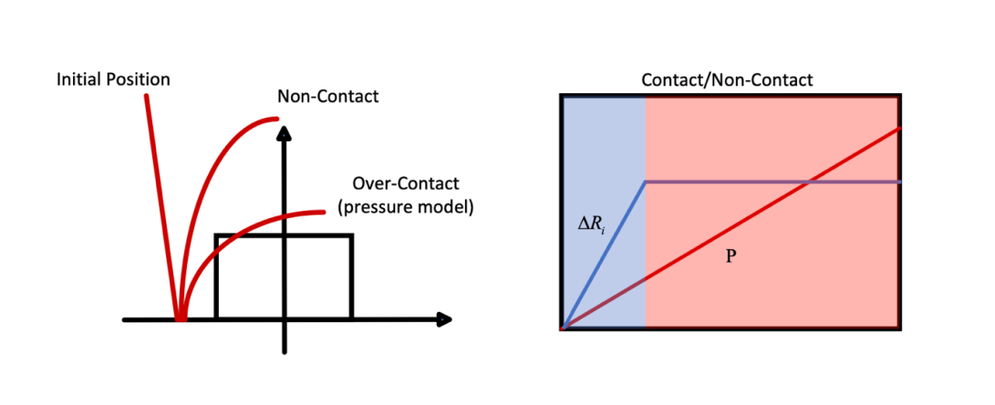
Figure 14: Comparison between Resistance model and Pressure Model and Contact Sensing method.

3.7. Size Estimation

In this section, a method of gripping-object size estimation is proposed based on the mathematical model of self-shape perception. As shown in Figure 15, the grasper will have an inclination angle as steady state without pneumatic pressure which is labeled \( β \) , and the length of each robotic finger is \( L \) . \( ({x_{a}},{y_{a}}) \) and \( ({x_{b}},{y_{b}}) \) are the end points of the grasper on a 2D plane, and \( q \) is the distance between the two fingers from the bottom. The top opening distance \( Q \) can be defined as:

\( Q=2(Lcos(π-β)) \) (30)

And the estimated diameter of the target can be defined by:

\( d=|{x_{b}}-{x_{a}}| \) (31)

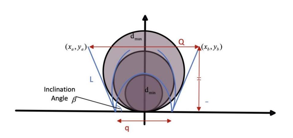
Figure 15: Illustration of the size estimation method

4. Experimentation

4.1. Model Accuracy Test

The model accuracy test is needed to test the accuracy of the mathematical model. A simulation of the model is created via MATLAB. The experiment starts with the collection of different deformations of the robotic fingers via pictures and record the according resistances from the sensors. One single robotic finger is fixed on a stand and the entire system connected with the computer recording the resistances sent from the sensors.

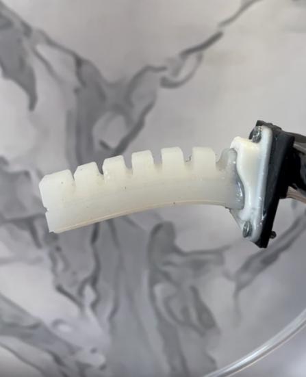
Figure 16: the robotic finger set on the stand.

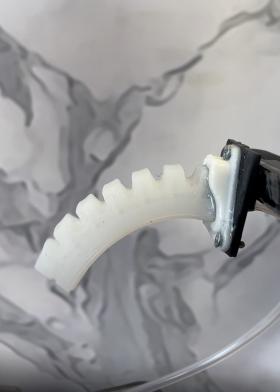
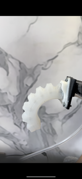
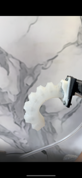
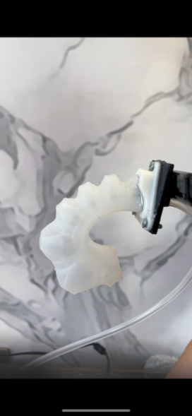
Figure 17: robotic finger deformation under the four experimental cases.

The following parameters for simulation were used. The total length L of the robotic fingers is 100mm. The thickness of \( {H_{0}} \) and \( {H_{1}} \) are 4mm and 11mm, respectively. The resistivity \( ρ \) is 0.0000073 \( Ω/m \) and \( {C_{10}} \) is 0.12 mPa. The simulation of the mathematical model then produces the following results:

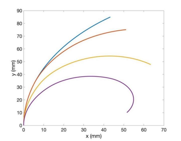
Figure 18: The simulation result based on the data from the robotic fingers.

The result showcases significant accuracy of the mathematical model in predicting the deformation of the robotic finger. The three-segment variational curvature model accounted for the increasing curvature to the end of the robotic finger due to more strain caused by pneumatic pressure which allows the model to be more accurate. In comparison, a single segment model would not account for this due to its single curvature output. The comparison between the simulation and the experimental data can be shown in the following picture:

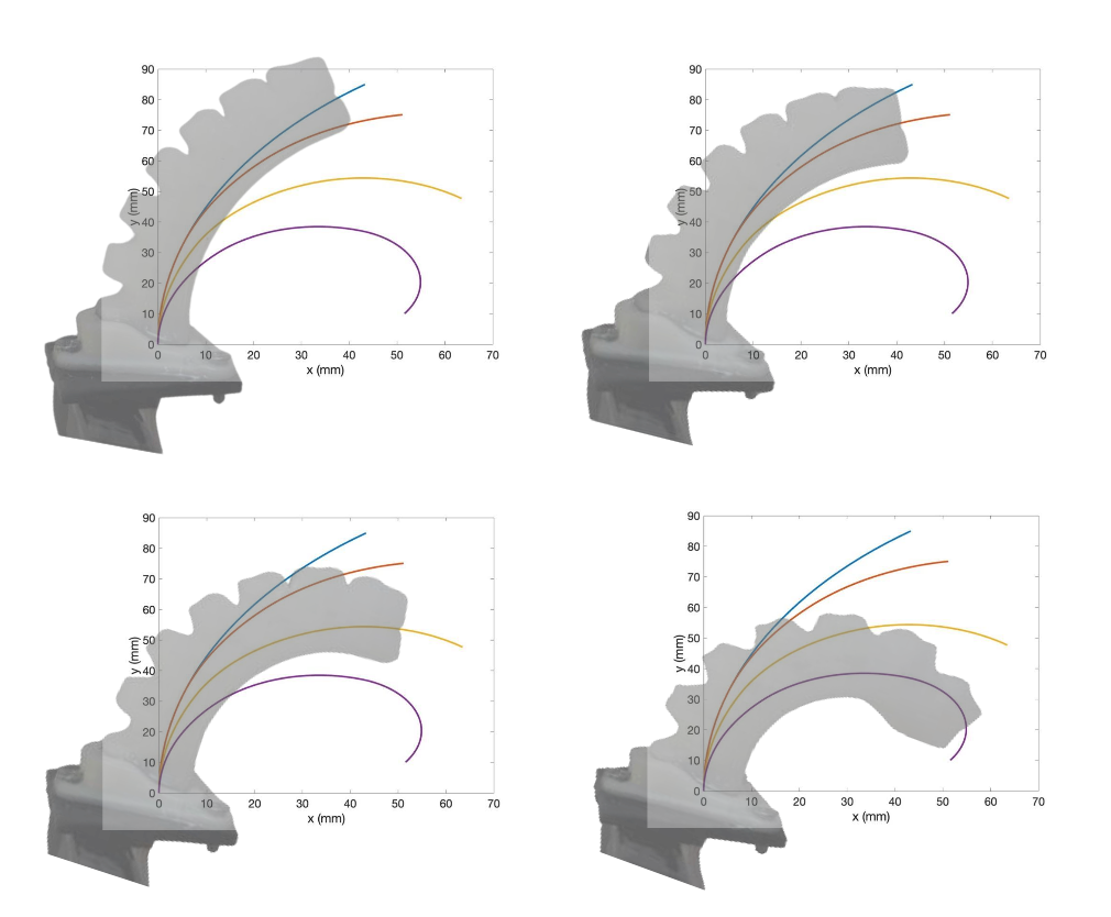
Figure 19: Comparison between experiment and simulation

4.2. Object Shape sensing Test

This section of the paper aims to test the validity of utilizing the model proposed to realize the gripping object shape sensing function.

The basic experimental setup is as the following figure:

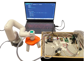
Figure 20: Experimental Setup

Where the robotic grasper is placed on a robotic arm that gives it the ability to move, and the grasper is also connected to the actuator and the computer to collect the resistance change data from the robotic fingers. The actuator was then given gripping objects of three shapes - circle, square, and triangle - with different sizes. Since the model is two-dimensional, the shapes are going to be axially elongated, which becomes cylinders, rectangular prisms, and triangular prisms.

In the experiment, I tested the grasper with five sizes for each shape and placed them in three different grip positions: upper, middle, and lower. With two of the robotic fingers integrated with the three-segment sensor, six different resistance signals were gathered in each trial.

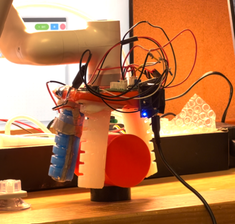
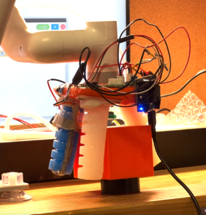
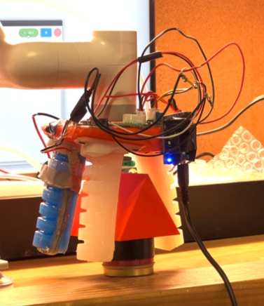
Figure 21: Gripping Experiment Cases

The experiment gathered a total of 45 six-dimensional data points. A statistical analysis is necessary to prove the validity of using this model in object-shape sensing to prove the significant differences between data points from each category since this provides the basis for a supervised learning model.

I used the multivariate analysis of variance (MANOVA) to analyze the differences between data points from different categories. MANOVA evaluates the mean vectors of different groups and determines if these vectors are significantly different, providing a more comprehensive understanding of group differences when multiple outcomes are considered. In the test, I chose to examine the four fundamental statistical data that reflects the differences between data: Wilks' lambda, Pillai's trace, Hotelling-Lawley trace, and Roy's greatest root, given by the following:

\( {Λ_{Wilks}}=\prod _{1~p}\frac{1}{1-{λ_{p}}}={det⁡(I-A)^{-1}} \) (32)

\( {Λ_{Pillai}}=\sum _{1~p}\frac{{λ_{p}}}{1-{λ_{p}}}={tr(I-A)^{-1}} \) (33)

\( {Λ_{LH}}=\sum _{1~p}{λ_{p}}=tr(A) \) (33)

\( {Λ_{Roy}}=\underset{ }{max}{(}{λ_{p}}) \) (34)

\( A=\frac{W}{B} \) (35)

Where W is the Within-Group Sum of Squares and Cross-Products Matrix, and B is the Between-Group Sum of Squares and Cross-Products Matrix. is the eigenvalue of the matrix A.

The result of the analysis is as follow:

Table 2: results from the MANOVA analysis

Notice that the p-value of the four species of data are lower than 0.05, which proves that the data tend to reject the null hypothesis and prove to be significantly different. The low p-value also provides a basis for further analysis based on the value of the four species. Wilk’s Lambda, with a significant p-value, proves more difference between data with a value closer to zero. In this case, the value is lower than 0.5, proving the data's differences. Pillai’s trace suggests the significance of differences with a value closer to 1, and in this case the value is greater than 0.5 which also proves the difference between data. The Hotelling-Lawley trace of around 1 and the Roy’s greatest root of 0.7474 also suggests the difference between data from different groups.

The great differences between the data for different gripping object shapes prove the validity of using machine learning in the future to realize the function of gripping object shape sensing.

5. Conclusions

The paper proposes a method of enabling “self-shape perception” for pneumatic soft robot. Based on the liquid metal composite sensor designed, the resistance signal collected will act as the input to the variational curvature model that estimates the deformation of the robotic finger. The process includes the fabrication of devices, construction of mathematical models, and experimentations to evaluate the performances of the system. The model can achieve self-shape perception, gripping object size estimation, and the detection of contact of the robotic finger. The last experiment validated the model’s ability to achieve object shape perception based on machine learning algorithms.

The experimentation in the paper still possesses numerous drawbacks. The lack of a professional experimentation setting and limits on experimenters and time caused problems such as the lack of large amount of quantitative data points which is not persuasive enough to prove a trend or relationship.

The contribution of the work mainly lies in the use of Ga-ln-Sn liquid metal composite as piecewise sensor for the robotic finger. Then, the mathematical model created to utilize the sensor to realize self-shape perception and other further applications to the robotic fingers. The meaning of the work does not merely lies in the creation of a model, but in a sense the work endowed the soft robotic graspers the ability to sense. It pushed the field of soft robotic studies from the level of structure to the level of intelligence, contributing to a process of improving from zero to one. The intelligent robotic grasper possesses numerous applications including mass production [9], human-machine interactions [10], and fragile item handling [11]. The elementary intelligence of the soft robots foresees a promising future of more advanced intelligence and even reaching the level of rigid-body robot today.

Beside the contribution and applications of the work, the process of research also benefitted me in many ways. In the process of completing the paper, I have practically gone through the whole process of researching a topic. All the steps from choosing a topic, searching for information, and writing this final paper have been a refining and sharpening of my thinking skills. During the process, I was able to scrutinize the concept of “scientific research” and was deeply impressed by its difficulty. I also encountered many difficulties and challenges in the process of experimentation, which made me deeply understand the importance of prudence when facing difficulties in different stages of my research and study.

References

[1]. S. Chen, H. Xu, F. Haseeb, W. Fan, and Q. Wei: Sens. Actuators, A 356 (2023). https://doi.org/10.1016/j. sna.2023.114284.
[2]. Y. Wang, H. Wang, and W. Chen: Jiqiren/Robot. 40 (2018) 5. https://doi.org/10.13973/j.cnki.robot.180378.
[3]. S. Shu, Z. Wang, P. Chen, J. Zhong, W. Tang, and Z. L. Wang: Adv. Mater. 35 (2023) 18. https://doi.org/10.1002/ adma.202211385.
[4]. Q. Shu, G. Liao, S. Liu, H. Deng, H. Pang, Z. Xu, X. Gong, and S. Xuan: Adv. Mater. Technol. 8 (2023) 2300019. https://doi.org/10.1002/admt.202300019.
[5]. Gianteye, “MakeSoftRobots / Kestrel / Kestrel_Mold_Core. STL at Master· Gianteye /MakeSoftRobots, ”GitHub, 2018, https://github.com/Gianteye/MakeSoftRobots/blob/master/Kestrel/Kestrel_Mold_Core.STL.
[6]. Z. Zhu, R. Zhao, B. Ye, and H. Wang: AIP Adv. 13 (2023) 115221. https://doi.org/10.1063/5.0158221.
[7]. Khaniki, H.B., Ghayesh, M.H., Chin, R. et al. A review on the nonlinear dynamics of hyperelastic structures. Nonlinear Dyn 110, 963–994 (2022). https://doi.org/10.1007/s11071-022-07700-3
[8]. F. Pineda, F. Bottausci, B. Icard, L. Malaquin, and Y. Fouillet: Microelectron. Eng. 144 (2015) 27. https://doi.org/10.1016/j.mee.2015.02.013.
[9]. A. Rajappan, B. Jumet, and D. J. Preston: Sci. Rob. 6 (2023) 51. https://doi.org/10.1126/scirobotics.abg6994.
[10]. Pan, M., Yuan, C., Liang, X., Dong, T., Liu, T., Zhang, J., Zou, J., Yang, H. and Bowen, C. (2022), Adv. Intell. Syst., 4: 2100140. https://doi.org/10.1002/aisy.202100140
[11]. Eduardo Navas et al., Frontiers in Robotics and AI 10 (January 18, 2024), https://doi.org/10.3389/frobt.2023.1330496.
Cite this article
Zhou,Z. (2025). Self-Shape Sensing Soft Pneumatic Grasper Based on Piecewise Liquid Metal Sensor and Piecewise Variational Curvature Model. Theoretical and Natural Science,83,51-69.
Data availability
The datasets used and/or analyzed during the current study will be available from the authors upon reasonable request.
Disclaimer/Publisher's Note
The statements, opinions and data contained in all publications are solely those of the individual author(s) and contributor(s) and not of EWA Publishing and/or the editor(s). EWA Publishing and/or the editor(s) disclaim responsibility for any injury to people or property resulting from any ideas, methods, instructions or products referred to in the content.
About volume
Volume title: Proceedings of the 4th International Conference on Computing Innovation and Applied Physics
© 2024 by the author(s). Licensee EWA Publishing, Oxford, UK. This article is an open access article distributed under the terms and
conditions of the Creative Commons Attribution (CC BY) license. Authors who
publish this series agree to the following terms:
1. Authors retain copyright and grant the series right of first publication with the work simultaneously licensed under a Creative Commons
Attribution License that allows others to share the work with an acknowledgment of the work's authorship and initial publication in this
series.
2. Authors are able to enter into separate, additional contractual arrangements for the non-exclusive distribution of the series's published
version of the work (e.g., post it to an institutional repository or publish it in a book), with an acknowledgment of its initial
publication in this series.
3. Authors are permitted and encouraged to post their work online (e.g., in institutional repositories or on their website) prior to and
during the submission process, as it can lead to productive exchanges, as well as earlier and greater citation of published work (See
Open access policy for details).