1. Introduction

With the increase in the world's population and the pollution of the environment, resources such as production resources, natural resources, etc., are becoming more and more limited. Under this circumstance, it is particularly important to find the optimal allocation of resources and use methods. Mathematical optimization methods are an important tool to solve such problems [1]. Mathematical Optimization is a branch of applied mathematics which is useful in many different fields, such as Manufacturing Production Inventory control, and so on [2]. With the development of technology, there are now many optimized methods. According to the objective function, optimization methods can be classified into linear and nonlinear optimization. When the objective function and all constraints are linear, the problem is classified as linear optimization. If the objective function or any constraint is nonlinear, the problem belongs to nonlinear optimization [3]. According to the domain of variables, optimization problems can be classified into discrete optimization and continuous optimization. In discrete optimization, the values of variables are finite or countable, such as in integer optimization problems. In continuous optimization, variables can take any value within a certain interval. According to the categories of parameters, optimization problems can be divided into deterministic and stochastic optimization. In deterministic optimization problems, all parameters are known and fixed, while in stochastic optimization (or stochastic programming), some parameters are random variables. According to the objective classification of optimization problems, we can divide them into single objective and multi-objective optimization. A problem that requires optimization of one objective function is called single objective optimization, while if there are multiple objective functions, it is called multi-objective optimization [4]. While many studies address these methods, limited work focuses on their comparative performance in real-world scenarios. In this paper, we will introduce several of the most widely used mathematical optimization methods based on optimization objects, optimization speed, optimization accuracy, etc., and analyze the advantages, disadvantages, and applicability of each method [5-7].

2. Gradient Optimization Methods

2.1. Gradient descent method

Gradient descent is one of the simplest and most widely used optimization method [8]. Its principles are easy to understand, making it widely applicable in various fields. However, the speed of gradient descent method is not the fastest. The method optimizes a function by iteratively moving in the direction of the steepest descent, defined as the negative gradient of the function at the current point. This property has earned it the alternate name of the “steepest descent method.” As shown in Figure 1, the closer the gradient descent method is to the target value, the smaller the step size becomes, leading to slower progress [9].

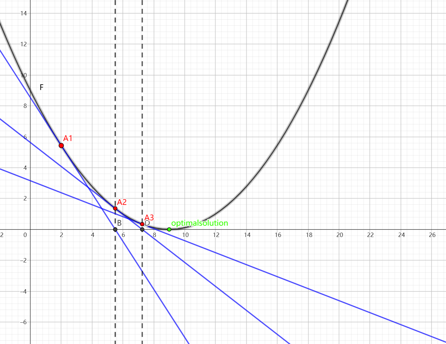
Figure 1: Diagram of Gradient Descent Method.

The gradient descent method has three disadvantages. First, the value of the step size will have a significant impact on the results. If the step size is too small, it will fall into local optimal and cannot find the global optimum. If the step size is too large, it will miss the global optimum. Second, the convergence speed of this method slows down when approaching the minimum value. Third, in the optimization process, it may decrease in a "Z-shaped" manner because the direction predicted by the gradient descent method is only the direction in which the function f decreases the fastest, not the direction towards the global optimal solution. This can cause the gradient descent method to fluctuate and decrease in a "Z-shaped" manner.

2.2. Batch Gradient Descent (BGD) method

The operation of batch gradient descent is to select S data points from the dataset as the training set. However, if the value of S is too small, it will result in large errors in the results and unsatisfactory optimization results. If the value of S is too large, it will result in calculating all S samples during each iteration, which will increase the computational workload and slow down the iteration speed. For cases where the sample size is not too large, the effect will be better, but for large-scale sample problems, the efficiency will be low. So, this introduces another method - stochastic gradient descent [10].

2.3. Stochastic gradient descent (SGD) method

The stochastic gradient descent method involves randomly selecting samples from a dataset for gradient descent analysis. This approach may result in lower accuracy compared to other methods and an increase in the number of iterations. However, when analyzing large-scale sample problems, the number of iterations added will be much smaller than the number of samples, leading to a significant improvement in overall optimization efficiency.

The results obtained by stochastic gradient descent are usually near the optimal solution. Overall, the overall idea of stochastic gradient descent is to sacrifice some accuracy in exchange for greater efficiency improvement. For large-scale sample analysis, this method will have a considerable effect [11].

2.4. Conjugate Gradient Method

In linear cases, the conjugate gradient method is applied to solve problems of the form Ax=b. When solving such problems, the best method is x = A-1b. However, when calculating in this way, it is inevitable to calculate the inverse of the matrix, which can be quite complex. Therefore, in the conjugate gradient method, we use an iterative method to solve it, which can simplify the calculation process. People have extended this method to nonlinear situations, which is called the nonlinear conjugate gradient method. Essentially, the idea of conjugate gradient method is to separately calculate the extremum of the objective function in different directions, and then combine them to obtain the extremum of the function. The conjugate gradient method accelerates convergence speed compared to gradient descent method by analyzing in different directions and avoids large-scale calculations of Newton's method. However, the conjugate gradient method only has superior performance in solving quadratic problems but performs poorly in other situations [12].

3. Newton's methods

3.1. Classical Newton's method

Newton's method is a method of approximating equations in both the real and complex domains. The general method uses the first few terms of the Taylor series of function f (x) to find the roots of equation f (x)=0. The biggest feature of Newton's method is its fast convergence speed.

The basic idea of Newton's method is to start from a point on the function f (x) that is closer to the solution, and find the intersection point between its tangent and the x-axis. The function value corresponding to the x-value at this point will be closer to the solution, and this process is repeated to find the solution of the function. Because Newton's method uses tangents to gradually approximate the solution of a function, it is also known as the tangent method.

Compared to the first-order convergence of gradient descent, Newton's method is a second-order convergence, second-order convergence, second order convergence will be such that each subsequent iteration will result in a factor of 2 reduction in the error between the optima and the current location [13]. So, it will have a faster speed in finding solutions. And Newton's method considers the global optimal solution, without the Z-shaped fluctuations of gradient descent, and the descent path will be more in line with the true optimal descent path.

However, Newton's method also has some drawbacks, such as the Strict requirements for functions (second-order continuous differentiability, reversible Hessian matrix), and in each iteration, it requires solving the inverse matrix of the Hessian matrix of the function, resulting in a considerable amount of computation. For the sake of simplicity in calculation, we have introduced the next method - the quasi-Newton method.

3.2. Quasi Newton method

The essential idea of the quasi-Newton method is to improve the defect of Newton's method which requires solving the inverse matrix of a complex Hessian matrix every time. It uses a positive definite matrix to approximate the inverse of the Hessian matrix, thereby simplifying the complexity of the operation [14].

4. Lagrange multiplier method

In some cases, instead of the objective function f(x) in equation (1), several functions, such as f1(x), f2(x), ..., fn(x), must be minimized simultaneously when solving the problem in the equation. This type of problem is called a multi-objective optimization problem [15], multi-objective optimization is common in everyday life [16]. and The Lagrange multiplier method is one of the main methods for solving constraint problems.

The basic Lagrange multiplier method with one constraint is a method of finding the extremum of function f under the constraint of g = 0. The basic operation is: if an extremum is taken at x0, the function must be tangent to the constraint condition, that is, there is only one intersection point, because if there are more than one intersection point, then that point is not an extremum point. If the function is tangent to the constraint condition, their normal vectors will be on the same line but in opposite directions. Represented by gradient vectors as Δ f (x0, y0) =λ Δ g (x0, y0), combined with the constraint of g (x0, y0) = 0, we can solve this system of equations, the process can be seen in figure 2 and obtain the solutions of the variables and the value of λ for the extremum of the original function. Where λ is the Lagrange multiplier [17]. For the general case, if we have n variables and k constraints, we can convert such an optimization problem into a solution to a system of equations with n + k variables by using the Lagrange multiplier method. The advantage of the Lagrange multiplier method is that it can transform conditional extremum problems into unconditional extremum problems and handle some multivariate problems. However, the extremum points found by the Lagrange multiplier method are not absolute and require further verification and judgment [18].

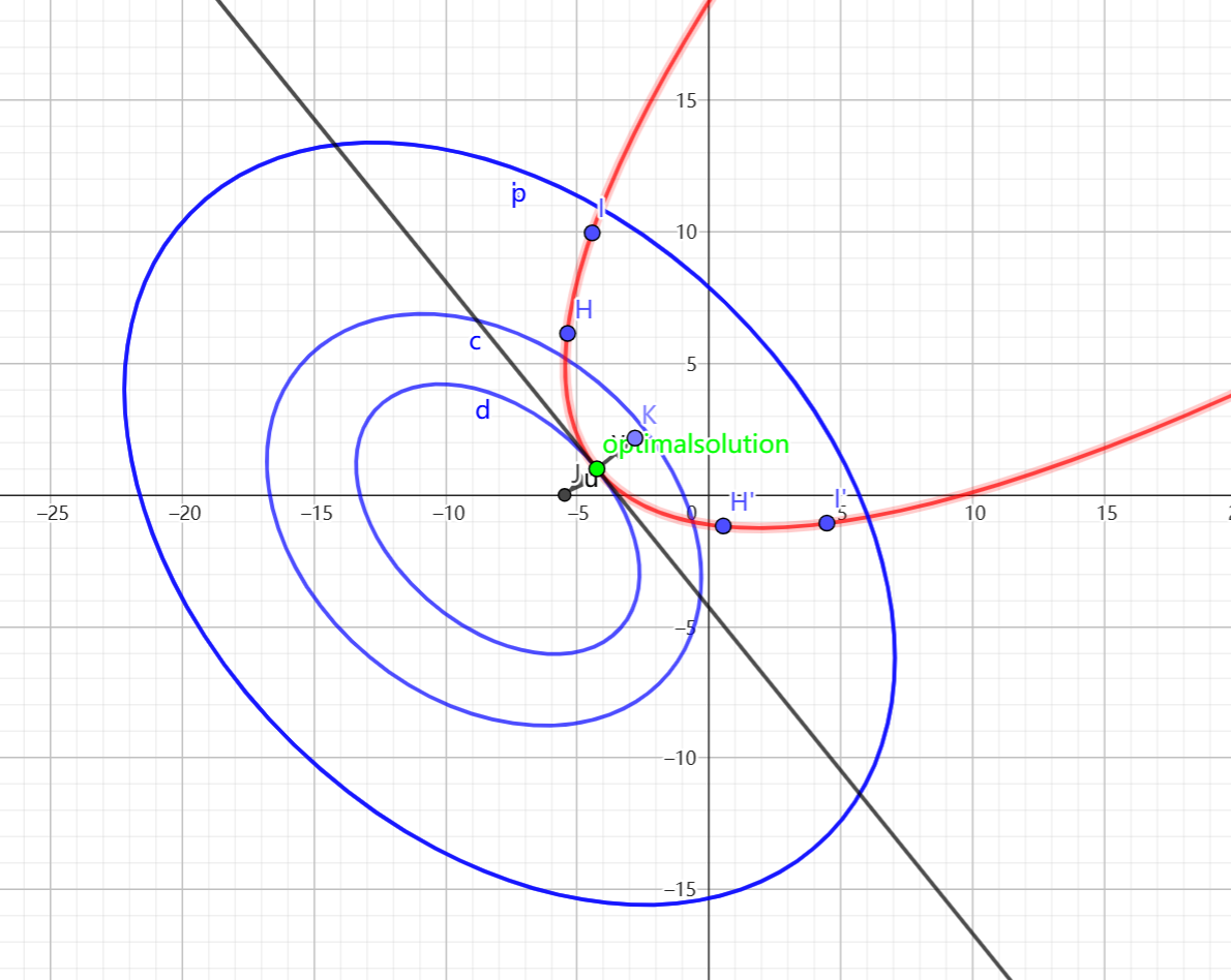
Figure 2: The diagram of Lagrange multiplier method.

5. Heuristic methods

It is obtained by simulating the development laws and working principles of things in nature, mainly including simulated annealing, ant colony algorithm, neural network and other algorithms.

Among the heuristic algorithms, one of the most representative and widely used is neural networks, A neural network is a program, or model, that makes decisions in a manner similar to the human brain, by using processes that mimic the way biological neurons work together to identify phenomena, weigh options and arrive at conclusions [19]. Neural networks are ideally suited to help people solve complex real-life problems, and have a significant impact in autonomous vehicles, voice-activated virtual assistants, medical imaging, and more [20].

The 2024 Nobel Prize in Physics was awarded to John J. Hopfield and Geoffrey Hinton for their foundational discoveries and inventions of machine learning for artificial neural networks, which are a testament to the importance of neural networks.

Usually, The Heuristic algorithms can use some information to predict and respond to calculations, making them an excellent heuristic method. And when searching for the optimal solution, there is a purpose rather than blindly searching for the optimal solution like other methods, which can quickly find the optimal solution. However, the design difficulty of heuristic algorithms can also be high, and the results of heuristic algorithms are random and difficult to predict.

6. Discussion

The gradient descent method is valued for its simplicity in both operation and principle. However, its major drawback lies in its slow convergence speed, and it may suffer from fluctuations during the descent process, leading to inefficiencies. The batch gradient descent method is more effective for problems involving smaller sample sizes, but it becomes inefficient when applied to large-scale datasets due to its computational complexity.

The stochastic gradient descent method (SGD), while less accurate and requiring a greater number of iterations compared to other methods, excels in handling large-scale problems. The added number of iterations in SGD is significantly smaller than the total number of samples, resulting in notable improvements in optimization efficiency for large datasets.

The Newton method offers the advantage of second-order convergence, faster processing speeds, and global optimization capabilities by considering the curvature of the solution space. However, its reliance on matrix calculations makes it computationally intensive, especially for high-dimensional problems. In contrast, the quasi-Newton method simplifies these calculations, reducing the computational burden while maintaining much of the efficiency of Newton’s method.

The Lagrange multiplier method is particularly useful for handling multivariate problems, making it suitable for constrained optimization scenarios. However, its results often require further verification to ensure accuracy and reliability.

The conjugate gradient method, compared to gradient descent, accelerates convergence while avoiding the computational intensity associated with Newton’s method. However, its effectiveness is primarily limited to solving quadratic problems, where it performs well, but it is less effective for non-quadratic problems.

Heuristic algorithms provide a different approach, excelling at quickly identifying optimal solutions even in complex optimization landscapes. Nevertheless, they are associated with high design complexity, and the resulting solutions may exhibit randomness and unpredictability, making them less reliable in certain scenarios.

Each mathematical optimization method has its unique strengths, limitations, and areas of applicability. The choice of the most suitable method depends on the specific problem context, balancing computational efficiency, accuracy, and complexity. Selecting the appropriate optimization method is crucial to achieving robust and efficient results.

7. Conclusion

Mathematical optimization methods are foundational tools with significant applications across a wide range of disciplines. In engineering, they contribute to enhancing product quality, conserving energy, reducing costs, and improving efficiency. In mathematics and computer science, optimization algorithms are essential for solving practical problems, while in fields such as machine learning, operations research, and economic forecasting, they enable robust decision-making and predictive modeling. Despite their extensive applicability, mathematical optimization methods are not without limitations. Real-world scenarios often deviate from the assumptions of idealized models, and computational errors can compromise the accuracy of the final results. These challenges underscore the need for continuous advancements to bridge the gap between theoretical models and practical applications [21] [22].

As Dr. Robert Bixby observed, the increasing availability and quality of data in recent decades have amplified the demand for mathematical optimization to support better decision-making. Among computational technologies, mathematical optimization stands out for its unparalleled robustness and ability to generate high-quality solutions [23].

Looking ahead, the development of mathematical optimization methods will focus on addressing current shortcomings in three key areas. First, enhancing the speed and functionality of solvers will accelerate optimization processes and expand their capacity to handle complex models. Second, improving the usability of optimization tools will make them accessible to non-specialists, enabling broader adoption and customization of models. Finally, increasing the accuracy of optimization results will ensure that solutions are more precise and better aligned with real-world conditions.

In conclusion, mathematical optimization methods will remain critical to tackling complex challenges in science, engineering, and beyond. By advancing solver performance, usability, and accuracy, the field can continue to drive innovation and support informed decision-making in an increasingly data-driven world.

References

[1]. Gurobi Optimization (Ed.) (2024) Mathematical Optimization: What You Need to Know. https://bit.ly/3COKkeV
[2]. Stanford University (Ed.) (2023) Introduction to Mathematical Optimization. https://bit.ly/3COvzc2
[3]. University of Washington (Ed.) (2022) https://bit.ly/3OlQRR2
[4]. Zhi Hu (Ed.) (2024) Optimization Theory Series: 3- Types of Optimization Problems https://bit.ly/3CCMJJE
[5]. China Association for Science and Technology (Ed.) (2013) Report on the Development of Operations Research Discipline of China Association for Science and Technology. https://bit.ly/3CIEBaM
[6]. Department of Chinese Academy of Science (Ed.) (2024) The Development Strategy of Chinese Disciplines Mathematical optimizationhttps://bit.ly/3YUvon6
[7]. Groetschel M. (2012). Extra Volume: Optimization Stories. Documenta Mathematica. https://bit.ly/3V4jdDf
[8]. Liang Wang. Jianxin Zhao. (2022) Mathematical Optimization. http://dx.doi.org/10.1007/978-1-4842-8853-5_4
[9]. Sebastian Ruder (2016, January,19) An overview of gradient descent optimization algorithms. ruder.io. https://doi.org/10.48550/arXiv.1609.04747
[10]. Inside Learning Machines (Ed.) (2024) What is Batch Gradient Descent? 3 Pros and Cons - Inside Learning Machines. https://bit.ly/4eJK3aG
[11]. Geeks For Geeks (Ed.) (2023) Difference between Batch Gradient Descent and Stochastic Gradient Descent. https://bit.ly/3OmSmOI
[12]. CSDN (Ed.) (2018) Nonlinear Optimization - Comparison of Several Optimization Methods (1)_ https://bit.ly/3CKq8Ly
[13]. MATHEMATIC (Ed.) (2020) What does first and second order convergence mean [with minimal equations] for optimization methods? https://bit.ly/4fFju7H
[14]. Wenjun Luo, Zezhong Wu, Shengyu He (2024). A class of improved quasi-Newtonian algorithms. http://dx.doi.org/10.16836/j.cnki.jcuit.2024.03.016
[15]. Science Direct (Ed.) (2015) Multiobjective Optimization. https://bit.ly/4i2Qb0k
[16]. Olivier L. DE WECK. (2003) MULTIOBJECTIVE OPTIMIZATION: HISTORY AND PROMISE. Massachusetts Institute of Technology. https://bit.ly/3B1wdm0
[17]. University of Maryland, College Park (Ed.) (2015) Lagrange multiplers and constraints. https://bit.ly/49aZVSshttps://bit.ly/49aZVSs
[18]. LibreTexts (Ed.) (2024) 2.7: Constrained Optimization - Lagrange Multipliers [18]https://bit.ly/40YY7ts
[19]. IBM (Ed.) (2021) What is a Neural Network? https://bit.ly/3YZBK4F
[20]. Coursera (Ed.) (2024) Neural Network Examples, Applications, and Use Cases | https://bit.ly/3AVxKKn
[21]. Lenstra J K, Rinnooy Kan A H G, Schrijver (1991). A. History of Mathematical Programming. https://doi.org/10.1007/BF00940190
[22]. National Research Council of the American Academy of Sciences. (2013) The Mathematical Sciences in 2025. https://doi.org/10.17226/15269.
[23]. Gurobi Optimization (Ed.) (2024) Mathematical Optimization: Past, Present, and Future. https://bit.ly/4ieLgKb
Cite this article
Zou,Y. (2025). Advancing Mathematical Optimization Methods: Applications, Challenges, and Future Directions. Theoretical and Natural Science,79,119-125.
Data availability
The datasets used and/or analyzed during the current study will be available from the authors upon reasonable request.
Disclaimer/Publisher's Note
The statements, opinions and data contained in all publications are solely those of the individual author(s) and contributor(s) and not of EWA Publishing and/or the editor(s). EWA Publishing and/or the editor(s) disclaim responsibility for any injury to people or property resulting from any ideas, methods, instructions or products referred to in the content.
About volume
Volume title: Proceedings of the 4th International Conference on Computing Innovation and Applied Physics
© 2024 by the author(s). Licensee EWA Publishing, Oxford, UK. This article is an open access article distributed under the terms and
conditions of the Creative Commons Attribution (CC BY) license. Authors who
publish this series agree to the following terms:
1. Authors retain copyright and grant the series right of first publication with the work simultaneously licensed under a Creative Commons
Attribution License that allows others to share the work with an acknowledgment of the work's authorship and initial publication in this
series.
2. Authors are able to enter into separate, additional contractual arrangements for the non-exclusive distribution of the series's published
version of the work (e.g., post it to an institutional repository or publish it in a book), with an acknowledgment of its initial
publication in this series.
3. Authors are permitted and encouraged to post their work online (e.g., in institutional repositories or on their website) prior to and
during the submission process, as it can lead to productive exchanges, as well as earlier and greater citation of published work (See
Open access policy for details).