1. Introduction

Humans’ exploration of the universe has never been weakened throughout history. After an arduous development of natural philosophy, people gradually realized that the universe follows specific patterns: for example, Kepler proposed his laws about planetary motion by analyzing Tycho Brahe's astronomical observations [1]. However, most findings, including Kepler’s laws, were empirical. Rather from serving as illustrations of more basic ideas, they were only invented to match with the findings of observations.

It was not until Newton published his epochal work Philosophiæ Naturalis Principia Mathematica that all the empirical were theoretically justified. Newtonian mechanics performed exceptionally well in solving two-body problems, where two objects move periodically around the system’s center of mass, and it also provided mathematical justification for Kepler’s laws and extended their application to more general situations. By studying forces between different objects, Newton successfully predicted celestial bodies’ motions. The prophecy and later discovery of Neptune in 1846 also proved Newton’s theories’ reliability[2]. The idea of a universal mechanism—that the entire cosmos is a painstakingly constructed machine—became eminent as a result of Newtonian mechanics' persuasive and fundamental nature.

Therefore, people after the 18th century firmly believed that everything was predictable and that the world was comprehensible. But can Newtonian mechanics completely unveil the secret of the universe? In 1885, Acta Mathematica held a prize competition in honor of King Oscar II that collected answers for the N-body problem. The final winner was French mathematician Henri Poincaré who devised a novel approach to problem-solving and seizing the chance to go deeper into the domain. Though he didn’t solve the problem, his contribution laid the foundation for other theories like chaos theory.

While Newtonian mechanics is impressive, it may not always be the most effective or singular approach, as illustrated by the challenges of the three-body problem. Another theory, analytical mechanics, was established after the efforts of numerous scientists, represented by Lagrange and Hamilton. It focuses on the system’s constraints and uses scalars to describe the system instead vectors, like forces in Newtonian mechanics. Also, since energy is more widespread than force, analytical mechanics could be more easily applied to statistical physics and quantum mechanics.

Mechanics has experienced a brilliant and twisting development. This paper is going to provide an loverview of the development of Newtonian mechanics through the lens of astronomy and offer a prediction for further research that will either build upon or be influenced by this field.

2. Newtonian mechanics

2.1. Kepler’s laws

Astronomy was well-developed before Newton’s time. Observing the universe has been a long-lasting tradition since recorded history began. A Danish astronomer, Tycho Brahe, meticulously observed planetary motions, particularly that of Mars, and provided accurate data [3]. His student Kepler spent 20 years analyzing his observation data and concluded three famous laws known as Kepler’s Laws from 1609 to 1619 [4]:

(1) The Law of Orbits: All planets move in elliptical orbits, with the sun at one focus.

(2) The Law of Areas: A line that connects a planet to the sun sweeps out equal areas in equal times.

(3) The Law of Periods: The square of the period of any planet is proportional to the cube of the semimajor axis of its orbit.

The laws are purely experimental. They were concluded from numerous data observed by Brahe. Before this discovery, Kepler attempted to search for the principle of planetary motion, but he focused not on Force but on “traditional scholastic doctrine inheriting Aristotelian metaphysics” [5] and designed a solar system model as shown in Figure 1 below:

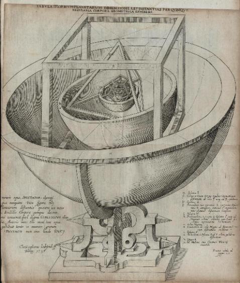
Figure 1: Solar System Model [6]

Kepler believed that the universe was harmonious and that all the planets moved along designated orbits around the sun, represented by different spheres in the model. However, Kepler’s laws disproved the previous models and did not find an explanation before Newton’s time.

2.2. Newton’s theories

In 1687, Isaac Newton used his laws of motion and laws of universal gravitation to justify Kepler’s law [7]. Kepler’s empirical conclusions are crucial, and extracting three concise formulas from numerous data was a magnificent work. However, Kepler did not connect his equations with the concept of force: the second law corresponds to the conservation of angular momentum and implies that the planets are subject to central force; the first law shows that the central force is the gravitational force, while the third law quantitively but indirectly implicates the magnitude of the force [8]. Therefore, by introducing the concept of force, Newton discovered the law of gravitation and the laws of motion, which are simpler and more fundamental and have further reach than Kepler’s planetary motion.

2.2.1. Central force

A central force on an object is a force that is directed towards or away from a point called center of force [9]. It has the form as follows:

\( F=f(r)\hat{r} \) (1)

\( \hat{r } \) is the position vector, and \( f(r) \) is a function that varies with changes of the object’s position. If \( f(r) \gt 0 \) , the central force is repulsive; if \( f(r) \lt 0 \) , the central force is attractive. Newton’s law of gravitation and Columb’s law are both inverse-square laws and deal with central forces.

2.2.2. Two-body motion

A two-body system is an isolated system of two particles that interact through a central potential [10]. It can usually be reduced to a one-body problem by using reduced mass: Considering two massive points with masses \( {m_{1}} \) and \( {m_{2}} \) , displacements at \( {r_{1}} \) and \( {r_{2}} \) respectively. Their center of mass has mass \( {m_{C}} \) and displacement \( {r_{C}} \) Since the system is isolated, the only forces between two massive points are their own interacting forces, supposed \( {f_{12}} \) and \( {f_{21}} \) , as \( {f_{21}}=-{f_{12}}=F \) According to Newton’s third law, we may derive:

\( \begin{matrix} & {m_{1}}\ddot{{r_{1}}}={f_{12}} \\ & {m_{2}}\ddot{{r_{2}}}={f_{21}} \\ \end{matrix} \) (2)

Adding the two equations we have:

\( {m_{C}}\ddot{{r_{C}}}=0 \) (3)

This equation suggests that the center of mass in a two-body system is either static or moving at a constant speed. Thus, if we take the center of mass as the origin (that is called the center of mass frame), the problem would be simplified. Suppose the positions of two points relative to their center of mass are \( {r_{C1}} \) and \( {r_{C2}} \) respectively:

\( \begin{matrix}{r_{C1}}={r_{1}}-{r_{C}}={r_{1}}-\frac{{m_{1}}{r_{1}}+{m_{2}}{r_{2}}}{{m_{1}}+{m_{2}}}=\frac{{m_{2}}}{{m_{1}}+{m_{2}}}({r_{1}}-{r_{2}}) \\ {r_{C2}}={r_{2}}-{r_{C}}={r_{2}}-\frac{{m_{1}}{r_{1}}+{m_{2}}{r_{2}}}{{m_{1}}+{m_{2}}}=-\frac{{m_{1}}}{{m_{1}}+{m_{2}}}({r_{1}}-{r_{2}}) \\ \end{matrix} \) (4)

Substitute \( {r_{1}}-{r_{2}} \) with \( r \) , the system is simplified to one-body form. Any of the two points can be chosen to build a frame of reference.

\( \ddot{{r_{1}}}-\ddot{{r_{2}}}=\frac{{f_{12}}}{{m_{1}}}-\frac{{f_{21}}}{{m_{2}}}=(\frac{1}{{m_{1}}}+\frac{1}{{m_{2}}})F=\frac{{m_{1}}+{m_{2}}}{{m_{1}}{m_{2}}}F \) (5)

Defining reduced mass \( μ=\frac{{m_{1}}{m_{2}}}{{m_{1}}+{m_{2}}} \) , we have an equation similar to Newton’s second law:

\( μ\frac{{d^{2}}r}{d{t^{2}}}=F \) (6)

Suppose the system has potential energy \( V(r) \) its mechanic energy \( E \) of the system is

\( E=\frac{1}{2}μ{v^{2}}+V(r) \) (7)

Where \( v \) is the speed of one body relative to another. This equation could be justified by adding the kinetic energy of each body in the center of mass frame and the potential energy \( V(r) \) .

Apparently, gravitational force is a kind of central force. From a more general perspective, this paper is going to study the trajectory of a massive point in a central force field.

2.2.3. Conservation of mechanical energy in a central force field

Suppose the mass of an object is \( m \) , and the central force exerted on it is \( F=f(r)\hat{r} \) According to Newton’s law:

\( m\ddot{r}=f(r)\hat{r} \) (8)

If we choose polar coordinates, the velocity of the object can be decomposed as:

\( v={v_{r}}\hat{r}+{v_{θ}}\hat{θ}=\dot{r}\hat{r}+r\dot{θ}\hat{θ} \) (9)

The second derivative can get the expression of acceleration in polar coordinates. Substitute \( \ddot{r} \) in (8) with the result. Because central force has no \( \hat{θ} \) component:

\( m(\ddot{r}-r{\dot{θ}^{2}})=f(r) \) (10)

\( m(2\dot{r}\ddot{θ}+r\dot{θ})=0 \) (11)

According to the conservation of angular momentum:

\( L=L\hat{L}=r×p=r×mv=r\hat{r}×m(\dot{r}\hat{r}+r\dot{θ}\hat{θ})=m{r^{2}}\dot{θ}(\hat{r}×\hat{θ}) \) (12)

Then let \( h={r^{2}}\dot{θ }, \) we have:

\( L=mh \) (13)

Eliminate \( \dot{θ} \) in (10) using (13):

\( m(\ddot{r}-\frac{{h^{2}}}{{r^{3}}})= f(r) \) (14)

Multiply \( dr \) on both sides and integrate:

\( \int _{{r_{0}}}^{r}m(\dot{r}d\dot{r}-\frac{{h^{2}}}{{r^{3}}}dr)=\int _{{r_{0}}}^{r} f(r)dr=V({r_{0}})-V(r) \) (15)

\( V \) represents the potential energy, and \( {r_{0}} \) is a random displacement in the field. It gives:

\( \frac{1}{2}m{r^{2}}+\frac{m{h^{2}}}{2{r^{2}}}+U(r)=\frac{1}{2}m{r^{2}}+\frac{m{h^{2}}}{2r_{0}^{2}}+V({r_{0}})=E \) (16)

Substitute \( h \) in (16) by \( {r^{2}}\dot{θ} \) we get the conservation of mechanical energy:

\( \frac{1}{2}m{r^{2}}+\frac{m{r^{2}}\dot{θ}}{2}+V(r)=E \) (17)

The second term could also be expressed as \( 1/2 I{ω^{2}} \) , where \( I \) is rotation inertia and \( ω \) is angular speed. According to 2.2.2, in the two-body problem, it is more meticulous in substituting \( m \) with \( μ \) , the reduced mass.

2.2.4. The Trajectory of a massive point

If we want to derive Kepler’s laws, we have to figure out the trajectory of the massive point. That could be mathematically calculated as follows [11]:

Combing and Rewriting \( h={r^{2}}\dot{θ} \) and (13):

\( L dt=m{r^{2}}dθ \) (18)

Take \( θ \) as a variable:

\( \frac{d}{dt}=\frac{dθ}{dt}\frac{d}{dθ}=\frac{L}{m{r^{2}}}\frac{d}{dθ} \) (19)

The substitution into (17) gives:

\( \frac{{l^{2}}}{2{mr^{4}}}{(\frac{dr}{ dθ})^{2}}+\frac{{l^{2}}}{2{mr^{2}}}+V(r)=E \) (20)

After rearrangement, it yields:

\( \frac{l dr}{{mr^{2}}\sqrt[]{\frac{2}{m}(E-V(r)-\frac{{l^{2}}}{m{r^{2}}})}}=dθ \) (21)

After integration, it becomes:

\( \int _{{r_{0}}}^{r} \frac{l dr}{{mr^{2}}\sqrt[]{\frac{2}{m}[E-V(r)-\frac{{l^{2}}}{m{r^{2}}}]}}+{θ_{0}}=θ \) (22)

If the function of potential energy \( V(r) \) is given, the equation of the trajectory can be calculated. Yet there is another way to figure out the trajectory equation without knowing \( V(r) \) but focusing on \( f(r) \) [12]:

Suppose \( u=\frac{1}{r} \)

\( \frac{du}{ dθ}=\frac{d}{dt}(\frac{1}{r})\frac{dt}{ dθ}=-\frac{\dot{r}}{{r^{2}}\dot{θ}}=-\frac{\dot{r}}{h } \) (23)

\( \frac{{d^{2}}u}{ d{θ^{2}}}=-\frac{1}{h}\frac{d\dot{r}}{ dt}\frac{dt}{ dθ}=-\frac{\undefinedaccchar168r}}{h\dot{θ}}=-\frac{\undefinedaccchar168r}}{{h^{2}}{u^{2}}} \) (24)

Combining (23), (24), (10), and \( h={r^{2}}\dot{θ } \) , it gives:

\( -m{h^{2}}{u^{2}}\frac{{d^{2}}u}{ d{θ^{2}}}-m{h^{2}}{u^{3}}=f \) (25)

This equation is Binet Equation: if \( f(r) \) is given, the trajectory of the massive point is known. In Kepler’s laws, the central force is gravitational force \( f=-G\frac{Mm}{{r^{2}}}=-GMm{u^{2}} \) . Substitute \( GMm \) with \( k \) , then \( f=-k{u^{2}} \) . The substitution into (25) gives:

\( \frac{{d^{2}}u}{ d{θ^{2}}}+u=\frac{k}{{mh^{2}}}=\frac{1}{l} \) (26)

Suppose \( l, ε \) are constants. If the angle is measured from the periapsis, then the general solution for the orbit is:

\( lu=1+ε cosθ \) (27)

The above polar equation describes conic sections [13]. Since \( u=\frac{1}{r} \) :

\( r=\frac{l}{1+εcos⁡θ} \) (28)

Where \( l \) is latus rectum and \( ε \) is orbital eccentricity. The nature of the orbit depends upon the magnitude of e according to the following scheme [14]:

\( ε=0, circle \)

\( 0 \lt ε \lt 1, ellipse \)

\( ε=1, parabola \)

\( ε \gt 1, hyperbola \)

Therefore, in Kepler’s first law, \( 0 \lt ε \lt 1, \) and a planet moves along an elliptical orbit. Also, the property of conic section tells that the ellipse has a principal axis of length \( 2a=\frac{2l}{1-{ε^{2}}} \) , so \( a=\frac{l}{1-{ε^{2}}} \) . The period of planets orbiting the sun is:

\( T=\frac{2πab}{h}=\frac{2π{l^{2}}}{h{(1-{ε^{2}})^{\frac{3}{2}}}} \) (29)

Therefore, Kepler’s Third Law is justified:

\( \frac{{T^{2}}}{{a^{3}}}=\frac{4{π^{2}}l}{{h^{2}}}=\frac{4m{π^{2}}}{k}=constant \) (30)

In conclusion, Newton’s theory achieved enormous success in establishing a general, complete, and systematic law of the universe. Its application is widespread not only in astronomy but almost in every field of science. After centuries of improvement and supplement, it has been exceptionally well-developed and almost unimpeachable. Newtonian mechanics dominated the contemporary view of the universe, urging people to believe that the universe works strictly under natural laws and is like a precise clock or machine. Such a perspective is called a “universal mechanism”. French mathematician Laplace even conceived an intellect which at some point would be aware of every force causing nature to move as well as every location of every component that makes up nature.Nothing would be unclear, and it might be able to see both the past and the future right before it. [15] In other words, if one knows the very accurate state of the present, then both the future and the past become fully accessible.

3. Beyond Newtonian mechanics

3.1. Three-body problem

Although Newton’s theory can correctly express the interaction among many objects, solving them is not guaranteed: as shown in 2.2 above, finding the way to solve real problems is much more complicated than listing basic equations. Thus, the universe could be a machine, but it could never be completely understood, at least for humans, since scientists cannot figure out the accurate function of motion. The three-body problem is a representative example of that.

Similar to the two-body problem, the three-body problem describes three masses interacting

through Newtonian gravity without any restrictions imposed on the initial positions

and velocities of these masses [16]. The Newtonian equations are easy to give:

\( {\undefinedaccchar168r}_{1}}=-G{m_{2}}\frac{{r_{1}}-{r_{2}}}{{|{r_{1}}-{r_{2}}|^{3}}}-G{m_{3}}\frac{{r_{1}}-{r_{3}}}{{|{r_{1}}-{r_{3}}|^{3}}} \) (31)

\( \begin{matrix} & \\ & {\undefinedaccchar168r}_{2}}=-G{m_{3}}\frac{{r_{2}}-{r_{3}}}{{|{r_{2}}-{r_{3}}|^{3}}}-G{m_{1}}\frac{{r_{2}}-{r_{1}}}{{|{r_{2}}-{r_{1}}|^{3}}} \\ & \\ \end{matrix} \) (32)

\( {\undefinedaccchar168r}_{3}}=-G{m_{1}}\frac{{r_{3}}-{r_{1}}}{{|{r_{3}}-{r_{1}}|^{3}}}-G{m_{2}}\frac{{r_{3}}-{r_{2}}}{{|{r_{3}}-{r_{2}}|^{3}}} \) (33)

Newton discussed a special case of a three-body problem in Principia [17]. But a three-body problem does not have general solutions, because unlike a two-body problem, the three-body problem could not be simplified by reducing it to a one-body problem. This was proved by Poincaré that three-body and N-body problems have no real analytic integral [18].

Three-Body Problem was developed throughout the 18th and 19th centuries by Euler, Clairaut, d’Alembert, Laplace, Lagrange, Jacobi, Cauchy, etc. However, it was not until the end of the nineteenth century that Poincaré opened a new era, introducing geometric, topological, and probabilistic methods to understand qualitatively the incredibly complicated behavior of most of the solutions to this problem. By investigating the three-body problem, Poincare published his monumental essay New Method of Celestial Mechanics, which became the foundation of chaos theory. Poincaré discovered that the solution to the three-body problem is unbelievably complicated, making it impossible to predict the final state of the orbit under given conditions. After years, mathematicians discovered such unstable states are common in dynamic systems, and they called such systems “chaotic” [19]. While traditional science deals with supposedly predictable phenomena, chaos theory deals with nonlinear things that are impossible to predict, like turbulence, heartbeat irregularities, and road traffic [20]. A famous example is the butterfly effect: a butterfly flapping its wings in Brazil can cause a tornado in Texas. This metaphor shows the uncertainty of the chaotic system. Anyway, the emergence of chaos theory tells people that the future is unpredictable and the universe is still mysterious and sophisticated.

The mathematical approach to solving the three-body problem is complex and indirect. However, with modern computer simulation technology, a direct illustration of a chaotic system’s complexity could be given. With specific \( x,y, and z \) coordinates of three points, their trajectories could be drawn as illustrated in Figure 2;and If the z coordinate changed by 0.000001, it yields an entirely different graph as shown in Figure 3:

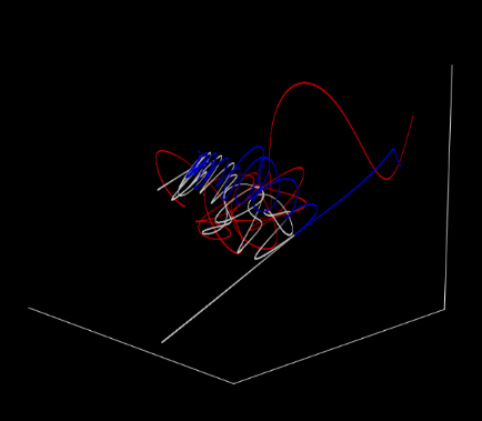
Figure 2: Trajectories of Three Body Motion [21]

If the z coordinate changed by 0.000001, it yields an entirely different graph as shown in Figure 3:

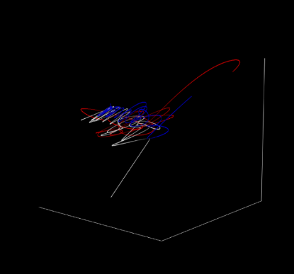
Figure 3: Trajectories of Three Body Motion After A Little Change [21]

3.2. Analytical Mechanics

As was mentioned at the end of 2.2.4, Newtonian mechanics gained huge success by using mathematical approaches to explain multifarious phenomena in the natural world. However, Newtonian mechanics focuses on the concept of “force”, which may not be the only and the perfect choice. Instead, after years of effort by scientists represented by Lagrange and Hamilton, a new theory was established: analytical mechanics. It focuses on scalar properties of motion, usually energy, while Newtonian mechanics focuses on vectors. Under chaotic circumstances, like the three-body problem, Newtonian mechanics is hard to apply.

Newtonian mechanics is familiar with displacement \( r \) that designates the relative position of a point in a three-dimensional world, and \( v, a \) are acquired henceforth. However, in analytical mechanics, generalized coordinates are adopted: They no longer rely on the displacement of massive points but on other independent parameters, the number of which is defined by the system’s degrees of freedom [21]. For a given system, the degrees of freedom are fixed. For a massive point, its position in 3-dimensional space is described by three components: \( x,y, and z \) . Therefore, the degree of freedom for this point is 3. When adding another independent point, the degree of freedom of the system is 6. The three new independent parameters could either be \( {x^{ \prime }},{y^{ \prime }}, and {z^{ \prime }} \) , or the distance between two points \( d \) , polar angle θ, and azimuthal angle φ, like in spherical coordinate. The two expressions are entirely equivalent. Analogously, the general coordinates ensure the coherence of degrees of freedom but choose other parameters to describe the state of the system. Such an operation may simplify the problem by jumping out of the restriction of spatial coordinates and make it easier to solve problems.

Noticeably, analytical mechanics is equivalent to Newtonian mechanics, and the scope of its application is not wider than that of Newtonian mechanics. In analytical mechanics, a mechanical system is characterized by function \( L({q_{1}},{q_{2}}…{q_{s}},\dot{{q_{1}},}\dot{{q_{2}}}…\dot{{q_{s}}},t) \) such that

\( S=\int _{{t_{1}}}^{{t_{2}}} L(q,\dot{q},t)dt \) (34)

takes the least value (Hamilton’s principle) and \( L \) is called Lagrange’s function, in many cases expressed as \( T-V \) , where \( T \) is the system’s kinetic energy and \( V \) is the potential energy [22]. After mathematical manipulation, it yields \( s \) equations:

\( \frac{d}{dt}(\frac{∂L}{∂{\dot{q}_{i}}})-\frac{∂L}{∂{q_{i}}}=0 (i=1,2,…,s) \) (35)

Which are the differential equations of the motion, called Lagrange’s equation. These concepts are fundamental in analytical mechanics: they express Newtonian mechanics from a novel perspective and have advantages over it.

Indeed, analytical mechanics may seem harder to comprehend compared with intuitive concepts like force. However, it is human’s natural inclination to shift from the intuitive to the abstract, from special to general, and from the ordinary l to the transcendental.

4. Conclusion

In summary, Newtonian mechanics forms a critical part of humanity's understanding of the cosmos, because it provides a methodical approach to deciphering the movement of celestial objects and the forces governing them. The understanding of physics was revolutionized by Newton's laws, which also made it possible to explain Kepler's empirical planetary observations and foster progress across other scientific fields. Yet, despite its monumental impact, Newtonian mechanics encountered limitations, especially when addressing intricate problems such as the three-body issue, which called for the application of alternative methodologies. The advent of analytical mechanics and chaos theory broadened the scope of our knowledge, addressing systems that defy straightforward prediction. Specifically, analytical mechanics introduced a fresh, energy-centric framework for comprehending motion, simplifying the complexities of many dynamic systems. While Newtonian mechanics holds an esteemed place in the history of science, it represents just a fraction of the ongoing quest to decode the universe, paving the way for successive theories that continue to refine the understanding of the cosmos and the laws governing it. This ongoing procedure serves as an example of how scientific research is constantly changing, with each new discovery building on the work of earlier ones.

References

[1]. Holton, G.J., Brush, S.G. (2001) Physics, the Human Adventure: From Copernicus to Einstein and Beyond. Rutgers University Press, Piscataway, NJ.
[2]. Kollerstrom, N. (2007) A Neptune Discovery Chronology: The British Case for Co-prediction. https://web.archive.org/web/20051119031753/http://www.ucl.ac.uk/sts/nk/neptune/chron.html. Accessed September 17, 2024.
[3]. University of Rochester. (n.d.) The Observations of Tycho Brahe. https://www.rochester.edu. Accessed September 17, 2024.
[4]. HyperPhysics. Kepler's Laws. https://hyperphysics.phy-astr.gsu.edu/hbase/kepler.html. Accessed December 13, 2022.
[5]. Sunada, T. (2016) From Euclid to Riemann and Thereafter. ResearchGate. https://doi.org/10.13140/RG.2.1.3809.5444.
[6]. Kepler, J. (1604) Astronomica Pars Optica. https://archive.org/details/den-kbd-pil-22002200031E-001/page/n50/mode/2up?view=theater. Accessed September 17, 2024.
[7]. Britannica, T. Editors of Encyclopaedia. (2019) Who Did Johannes Kepler Influence? https://www.britannica.com/question/Who-did-Johannes-Kepler-influence. Last modified June 21, 2019.
[8]. University of California, Davis. (2022) Kepler’s Laws. https://phys.libretexts.org/@go/page/18419. Last modified November 9, 2022.
[9]. Taylor, J.R. (2005) Classical Mechanics. University Science Books, Sausalito, CA.
[10]. Fratus, P. (2024) Three Body Problem. University of California Santa Barbara. https://web.physics.ucsb.edu/~fratus/phys103/LN/TBP.pdf. Accessed September 1, 2024.
[11]. Goldstein, H. (1950) Classical Mechanics. Internet Archive. https://archive.org/details/ClassicalMechanics. Accessed September 17, 2024. pp.87
[12]. Libretexts. (2024) Differential Orbit Equation. https://phys.libretexts.org/@go/page/9618. Last modified August 30, 2024.
[13]. Wikipedia. (n.d.) Binet Equation. https://en.wikipedia.org/wiki/Binet_equation#Classical. Accessed September 1, 2024.
[14]. Goldstein, H. (1950) Classical Mechanics. Internet Archive. https://archive.org/details/ClassicalMechanics. Accessed September 17, 2024. pp.94
[15]. Laplace, P.S. (1951) A Philosophical Essay on Probabilities. Dover Publications, New York.
[16]. Musielak, Z., Quarles, B. (2014) The Three-Body Problem. Reports on Progress in Physics, 77: 065901. https://doi.org/10.1088/0034-4885/77/6/065901.
[17]. Newton, I. (1729) The Mathematical Principles of Natural Philosophy. https://archive.org/details/NewtonPrincipia. Accessed September 17, 2024.
[18]. Yagasaki, K. (2024) A New Proof of Poincare’s Result on the Restricted Three-Body Problem. arxiv.org. https://arxiv.org. Accessed September 1, 2024.
[19]. Hasselblatt, B., Katok, A. (2003) A First Course in Dynamics: With a Panorama of Recent Developments. Cambridge University Press, Cambridge.
[20]. Fractal Foundation. What is Chaos Theory? https://fractalfoundation.org/resources/what-is-chaos-theory/. Accessed September 17, 2024.
[21]. Badger, B. The Three-Body Problem. Accessed September 17, 2024. https://blbadger.github.io/3-body-problem.html.
[22]. Amirouche, F.M.L. (2006) Fundamentals of Multibody Dynamics: Theory and Applications. Springer, Berlin.
[23]. Landau, L.D., Lifshitz, E.M. (1976) Mechanics. 3rd ed. Vol. 1. Butterworth-Heinemann, Oxford
Cite this article
Ye,X. (2025). Navigating the Cosmos: The Evolution and Impact of Newtonian Mechanics. Theoretical and Natural Science,87,26-35.
Data availability
The datasets used and/or analyzed during the current study will be available from the authors upon reasonable request.
Disclaimer/Publisher's Note
The statements, opinions and data contained in all publications are solely those of the individual author(s) and contributor(s) and not of EWA Publishing and/or the editor(s). EWA Publishing and/or the editor(s) disclaim responsibility for any injury to people or property resulting from any ideas, methods, instructions or products referred to in the content.
About volume
Volume title: Proceedings of the 4th International Conference on Computing Innovation and Applied Physics
© 2024 by the author(s). Licensee EWA Publishing, Oxford, UK. This article is an open access article distributed under the terms and
conditions of the Creative Commons Attribution (CC BY) license. Authors who
publish this series agree to the following terms:
1. Authors retain copyright and grant the series right of first publication with the work simultaneously licensed under a Creative Commons
Attribution License that allows others to share the work with an acknowledgment of the work's authorship and initial publication in this
series.
2. Authors are able to enter into separate, additional contractual arrangements for the non-exclusive distribution of the series's published
version of the work (e.g., post it to an institutional repository or publish it in a book), with an acknowledgment of its initial
publication in this series.
3. Authors are permitted and encouraged to post their work online (e.g., in institutional repositories or on their website) prior to and
during the submission process, as it can lead to productive exchanges, as well as earlier and greater citation of published work (See
Open access policy for details).