1. Introduction

Year after year, the frequency and impact of heavy rain disasters increase due to ongoing global climate change and urbanization. Disasters caused by heavy rain are abrupt, powerful natural events that cause major damage and losses to urban areas [1]. China has fewer than 3 trillion m³ of total water resources, yet only 0.22 thousand m³ of water resources are available per person, 0.25 times the average global level [2]. However, although Guangzhou has a large population base, its per capita water resources amount to only 0.2 times the national average, categorizing it as a region with extremely scarce water resources.

In recent years, extreme precipitation events have become frequent in Guangzhou. On May 7, 2017, the city experienced a rare historical downpour, transitioning from heavy rain to torrential rain. In Yongning Street, Zengcheng, the rainfall reached 382.6 millimeters in just three hours.In April 2024, the Guangzhou Climate and Agricultural Meteorology Center reported that the average monthly rainfall in the city reached 669.2 millimeters, which is an abnormal increase of 219.1% compared to the same period in previous years, breaking the historical record for rainfall during this time.The Lütian Lianma Meteorological Observation Station in Conghua District recorded a total rainfall of 1491.3 millimeters in April, breaking the monthly rainfall record for all months in Guangzhou since 1951.Against the backdrop of global warming, the tropical high pressure has been persistently shifting westward and intensifying, resulting in abundant moisture transport. The moisture conditions over Guangdong are very favorable, leading to intense and prolonged precipitation events this year, with overlapping affected areas, significantly increasing disaster risks and causing severe damage locally.

This article first conducts a preliminary visual analysis of the sequence characteristics of precipitation in Guangzhou from 2006 to 2023, and performs data processing such as handling missing values and frequency transformation.Next, I will explain the research methods involved in this article, followed by modeling the sequence using two types of models: the classic ARIMA and regression functions. Finally, I will use two forecasting methods, Basic-bootstrap and Full-bootstrap, to predict the precipitation for the next year based on the two estimated models.

According to the analysis, this article found that the regression model had the best Full bootstrap prediction performance, and the remaining three prediction results all had some deviation issues, especially in April when extreme precipitation occurred in Guangzhou this year. The two classic ARIMA prediction results were both low, so the model's estimation of precipitation extremes was inaccurate. It is considered that the problem of parameter cancellation in the MA coefficient during the process of the classic SARIMA model, as well as the problem of first-order seasonal differences, led to significant deviation in the prediction results. The reason why the regression model is generally better than the ARIMA model and the Basic bootstrap model has slightly inferior prediction performance is considered to be due to the shortcomings of the method itself, which is that the prediction method is not complete and scientific enough. During the bootstrap sampling process, only the residuals of the model are sampled, which has certain shortcomings in the sampling method. The Full bootstrap method just fills the gap in the sampling method of the former.

2. Method

2.1. Data Overview and Preprocessing

2.1.1. Basic Information and Feature Analysis of Data

This article collects daily precipitation data from the Guangzhou area from January 2006 to May 2024, measured in millimeters. The original data length is 6574, with a frequency of 365. After frequency conversion processing, the data length is 216, with a frequency of 12.The data came from the National Environmental Information Centre (NCEI) under the National Oceanic and Atmospheric Administration (NOAA).

The original sequence has missing values, and there is no obvious pattern in the distribution of the missing data; it is believed that the occurrence of these missing values is random. Figure 1 shows the time series plot and ACF plot of the original sequence. In the left graph, it can be observed that the range of the data is quite large, overall it is relatively dispersed, and there are noticeable periodic fluctuations. The right image shows a waveform similar to sine and cosine, and there is no trend of attenuation. A preliminary judgment suggests that seasonality is one of the reasons for the strong long-term memory.

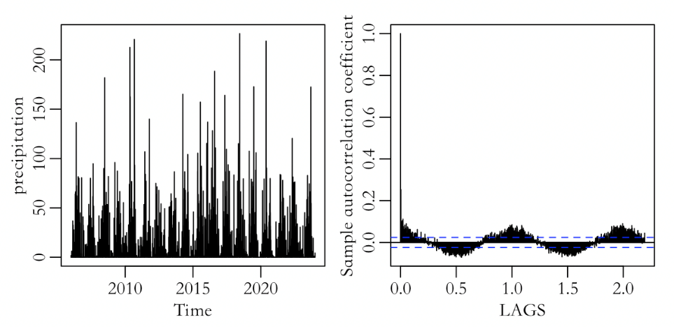
Figure 1: Daily frequency time series chart of the original sequence (left), Daily frequency ACF chart of the original sequence (top right).

2.1.2. Missing Data Imputation and logarithmic, Frequency Transformation.

For the handling of missing values, firstly, due to the special nature of precipitation values always being greater than or equal to 0, and the unpredictability of whether it rained on that day, the missing data is filled with 0. Secondly, there are a large number of values in Figure 1 that are around 0 and have large extreme values, resulting in scattered data overall. In subsequent ARIMA modeling, since the fitted results of the model randomly traverse the entire real number domain, precipitation data cannot be less than 0. In order to eliminate this asymmetry, logarithmic transformation is applied to the data. The transformed sequence distribution is significantly more concentrated, and even negative values are reasonable in the subsequent modeling and prediction process. The two ACF plots in Figure 2 also clearly show waveforms similar to sine and cosine functions. In order to study their seasonality, daily frequency data was converted into monthly frequency data.

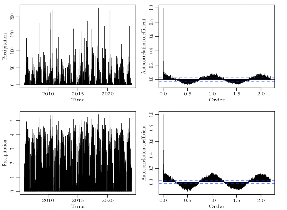
Figure 2: the daily frequency time series plot after filling in missing values (top left) and the daily frequency ACF plot (top right), the log-transformed daily frequency time series plot (bottom left), and the log-transformed daily frequency ACF plot (bottom right).

2.2. Research Method

2.2.1. Classic SARIMA Model

The ARIMA model is the abbreviation of autoregressive integral moving average model, which transforms non-stationary time series into stationary time series by differencing them, and then models them using autoregressive (AR) and moving average (MA) models. The general form of the ARIMA model is ARIMA (p, d, q), where p is the order of the autoregressive term, d is the differential order, and q is the order of the moving average term. Generally speaking, the seasonal parts of the series are characterized by \( (P,D,Q) \) , which may be expressed as follows, and the non-seasonal components of the series are illustrated by \( (p,d,q) \) in the SARIMA model, which is provided as \( SARIMA(p,d,q)(P,D,Q)s \) [3]:

\( {ϕ_{p}}(B){Φ_{P}}({B^{s}}){∇_{d}}∇_{s}^{D}{z_{t}}={θ_{q}}(B){Θ_{Q}}({B^{S}}){ℇ_{t}} \) (1)

2.2.2. Regression Model

This article uses a regression model based on sine and cosine functions (commonly referred to as seasonal decomposition model or seasonal adjustment model), which can decompose time series data into trend components, seasonal components, random components, etc., effectively capturing seasonal patterns and improving prediction accuracy.

In nonlinear regression models, growth curves are often an important model of study. Research indicates that regression prediction models based on trigonometric growth curves have a strong adaptability for fitting data, resulting in good fitting performance [4].

2.2.3. Basic Bootstrap Prediction

When the models under comparison are layered, the asymptotic distributions of the recursive out-of-sample forecast accuracy test statistics rely on stochastic integrals of Brownian motion. Because it is laborious to compute their asymptotic critical values, this frequently makes their practical implementation more difficult [5]. According to Monte Carlo simulations, the techniques work effectively with finite samples [6]. Only the residuals of the model are sampled with replacement, and historical values are used to predict the future, assuming that all uncertainties in the prediction come from white noise in the future. The coefficients of the prediction model are estimated using model coefficients and remain unchanged. Taking this article as an example, ARIMA(0,0,0)(0,1,1)(12):

\( \begin{cases} \begin{array}{c} {∇_{12}}{X_{t}}={Z_{t}} \\ {Z_{t}}={\hat{ϵ}_{t}}-0.9999998 {\hat{ϵ}_{t-12}} \end{array} \end{cases} \) (2)

Among them, \( {\hat{ϵ}_{1}} \) to \( {\hat{ϵ}_{216}} \) are model residuals. Use Bootstrap method to make predictions for the next 12 periods of the model. Predict based on residual estimation and historical data, using MAQ, ARP, and RWD functions. The development of simulation sequences in the next 12 periods - simulation \( {x_{205}},{x_{206}},...,{x_{216}} \) . According to the expression of the model, simulate the values \( {z_{205}},{z_{206}},...,{z_{216}} \) of the MA (12) component, finally simulate the values \( {x_{205}},{x_{206}},...,{x_{216}} \) ,... of RW (12) component.

2.2.4. Full Bootstrap Prediction

The sentence must end without a period. It is believed that residuals have uncertainty, and the estimated model parameters themselves also have uncertainty. Therefore, taking this article as an example, it is not only necessary to perform replacement sampling on the model residuals, but also to obtain 216 new samples by performing replacement sampling on the estimated model residuals with a sequence length of 216 times. Then, ARIMA modeling should be performed again on these samples to obtain more reasonable model coefficients. Perform a 12 period replacement sampling on the residuals of the new model and predict the values for the next 12 periods.

2.3. Model Selection

2.3.1. Classic SARIMA Model

One benefit of the SARIMA approach is that it can finish linear datasets [7]. Sequence stationarity judgment - Based on the time sequence diagram of the logarithmic frequency sequence in Figure 3, it can be determined that the sequence has no trend, that is, there is no instability caused by random trends, and there are no unit roots, so ordinary differencing is not performed. However, due to the obvious sine and cosine like waveforms in the ACF graph in the upper right of Figure 3, there is seasonal instability, so seasonal differentiation is performed on the sequence. Due to the seasonality of the sequence, the ADF unit root test results are not reliable, so the "ADF unit root test" is no longer used to support the above analysis.

As shown in the ACF diagram at the bottom right of Figure 3, the seasonality of the sequence after seasonal differentiation no longer exists, eliminating seasonal instability. The obvious first-order truncation of the season, the following modeling process first considers using ARIMA (0,0,0) (0,1,1) (12). (Note: The ACF chart clearly shows a first-order negative correlation between seasons, which will be discussed at the end of the ARIMA model.)

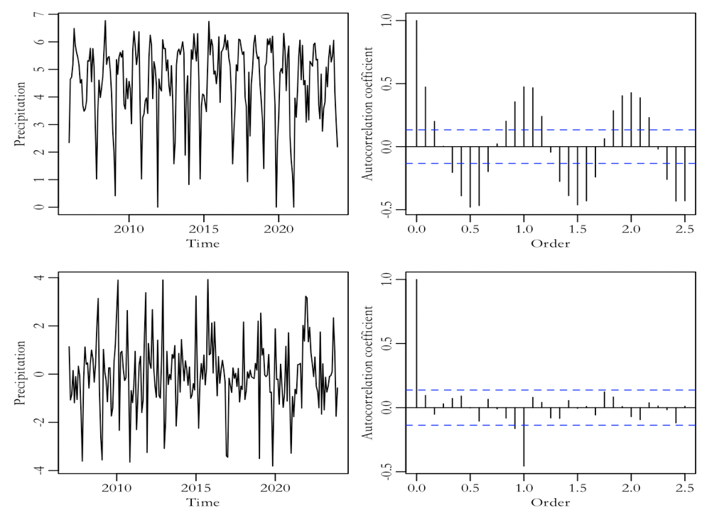
Figure 3: Time series plot of the monthly logarithmic sequence (top left) and ACF plot of the logarithmic sequence (top right); time series plot of the seasonally differenced sequence (bottom left) and ACF plot after seasonal differencing (bottom right).

Based on the above analysis, establish the model ARIMA (0,0,0) (0,1,1) (12)

\( \begin{cases} \begin{array}{c} {∇_{12}}{X_{t}}={Z_{t}}+θ \\ {Z_{t}}={ϵ_{t}}-{b_{1}}{ϵ_{t-12}} \end{array} \end{cases} \) (3)

After verification, the residual is white noise, and the model passes the test. According to Table 1, the P-value of the MA coefficient is less than 0.05, which is significant, but the drift is not significant. Therefore, the model is improved and an ARIMA (0,0,0) (0,1,1) [12] model without drift term is established. The residual test of the improved model is white noise, and the model coefficients are significant. The MA coefficient here is -0.9999998, which is close to -1. There may be a problem of parameter cancellation, but it does not mean that the model is unusable in all cases. In some cases, such models may still be able to provide effective predictions, and the discussion on this issue is analyzed in the summary of this article.

Table 1: Coefficient estimation results of ARIMA(0, 0, 0)(0, 1, 1)(12).

2.3.2. Regression Model - Based on Sine and Cosine Functions

Linear regression stands as the prevalent statistical approach across numerous application domains, enabling the analysis of how a collection of explanatory variables influences a targeted response variable [8]. Firstly, use a regression function to fit the seasonality of the sequence, and use a trigonometric function that is also a periodic function to fit the seasonality. Simultaneously using both low-frequency and high-frequency trigonometric functions to achieve the goal of fitting complex periods. Based on experience, the maximum value of k in \( cos{(\frac{ktπ}{6})} \) is usually considered to be 3. Use the LM function to establish a regression model.

\( {X_{t}}={α_{0}}+{α_{1}}t+{β_{1}}cos({ω_{t}})+{γ_{1}}sin({ω_{t}})+{β_{2}}cos({2ω_{t}})+{γ_{2}}sin({2ω_{t}})+{β_{3}}cos({ω_{t}})+{γ_{3}}sin({ω_{t}})+{ϵ_{t}} \) (4)

The subscripts \( β \) and \( γ \) represent multiples and numbers of frequencies, respectively.

In the coefficient test of the regression model with 7 explanatory variables, only the coefficients of the intercept term \( {α_{0}} \) and \( {β_{1.1}} \) (cosine function with k value of 1) are significant. After removing insignificant coefficients and fitting again, Table 2 shows the coefficients of the improved regression model, all of which are significant. Therefore, the formula is:

\( {X_{t}}=4.55659-1.42866 cos({ω_{t}})+{ϵ_{t}} \) (5)

Seasonal modeling is completed, and the original sequence is subtracted from the regression model to obtain a sequence without seasonality. The ACF diagram in Figure 4 indicates that the sequence has no memory. Furthermore, white noise testing was performed on the sequence residuals, and it can be clearly seen in the right figure of Figure 4 that the P-values are all above the 0.05 threshold. The sequence residuals are white noise and no additional ARMA components need to be added.

Table 2: Regression model coefficients after removing insignificant terms.

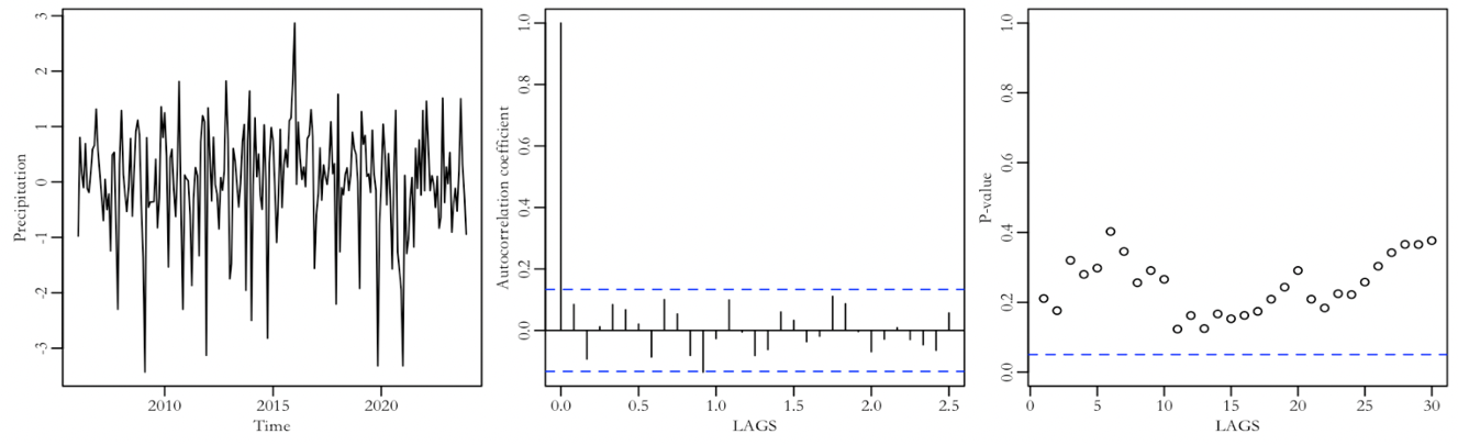
Figure 4: Time series plot of the seasonally adjusted series (left), ACF plot (middle), and P-value plot for white noise test (right).

3. Predictions

3.1. Basic Bootstrap Prediction

3.1.1. Based on the Classic SARIMA Model

Predict the precipitation for the next 12 periods, repeating the process 1000 times. The blue lines in Figure 5 represent the 97.5% upper bound, 2.5% lower bound, and mean of the 1000 predicted samples. The red line represents the latest actual precipitation data for the Guangzhou area from January to May 2024. The figure on the right shows that the majority of the actual data falls within the predicted range, but the actual precipitation in April exceeded the predicted range. The upper bound of the sample's 97.5% is 5.928503, and the actual value is 6.326672. The actual value exceeds its 97.5% upper bound, indicating that the model estimation is not accurate enough. Therefore, it is considered to improve and use the Full bootstrap model.

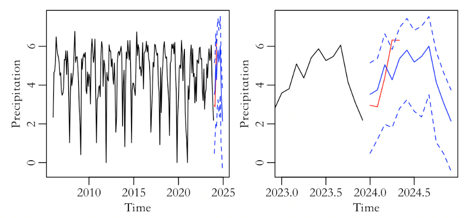
Figure 5: Time series plot of the ARIMA model including the latest data, predicted mean, and upper and lower bounds (left) and details of the left plot (right).

3.1.2. Based on Regression Model

The prediction process is analogous to the classic ARIMA modeling prediction process mentioned above. Figure 6 also compares the predicted results with the actual data, and it is clear from the right graph that the real data falls entirely within the predicted range. After comparing the specific values predicted by the two basic bootstrap models, it was found that the upper bound of the regression model was significantly larger and the prediction results were better. The regression model provides a more accurate prediction of the range of future precipitation, but the method of keeping the coefficients constant in Basic bootstrap prediction may result in the model's estimation not being the most scientific. Therefore, the more common Full bootstrap method will still be used for further prediction in the following text.

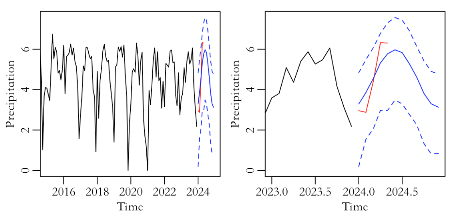
Figure 6: Time series graph of the regression model including the latest data, predicted mean, and upper and lower bounds (left) and details of the left graph (right).

3.2. Full Bootstrap Prediction

3.2.1. Based on the Classic SARIMA Model

The blue and red lines in Figure 7 represent the same content as above. It can be seen from the figure that the data for April still exceeds the predicted range. The comparison between Basic prediction and Full prediction of ARIMA model shows that the upper bound of 97.5% in April is higher and closer to the true value under the Full bootstrap method. But the true value still hasn't completely fallen within the predicted range.

Therefore, it is preliminarily believed that the classical ARIMA model has poor prediction performance. Both prediction models exceeded the prediction interval in April, and although the MA coefficient of the models is significant, the value is close to -1, which is approximately believed to cause parameter cancellation. At the same time, as mentioned earlier, there was a situation of excessive seasonal differentiation during the first-order seasonal differentiation in the modeling process. Therefore, it is believed that the classical ARIMA model is not the best estimation model.

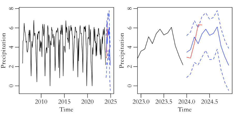
Figure 7: Time series graph under full-bootstrap with the latest data and predicted mean, upper and lower bounds (left) and details of the left graph (right).

3.2.2. Based on Regression Model

Table 3 shows the more reasonable new model coefficients estimated using the Full bootstrap prediction method, with the formula:

\( {X_{t}}=4.600298-1.392016 cos({ω_{t}})+{\hat{ϵ}_{t}} \) (6)

The real value in Figure 8 completely falls within the prediction range. At the same time, 2.5% of the full bootstrap prediction result of the regression model is almost improved in the next month with more precipitation compared with the full bootstrap data of the ARIMA model. The prediction range is accurate, and the upper bound value is larger in the rainstorm prone months, which is more in line with the actual situation. Compared with the two prediction methods of the regression model, the Full bootstrap prediction results effectively and reasonably narrowed down the prediction range, making it the best among the four prediction results. The occurrence of floods and waterlogging disasters in April 2024 brought great inconvenience to the Guangzhou area. This model is also more reasonable for predicting in April. Based on reality, if the predicted value is far lower than the actual value, it is not conducive to the relevant government departments planning and constructing urban drainage systems, nor is it conducive to making emergency plans in advance for the disaster (Table 3).

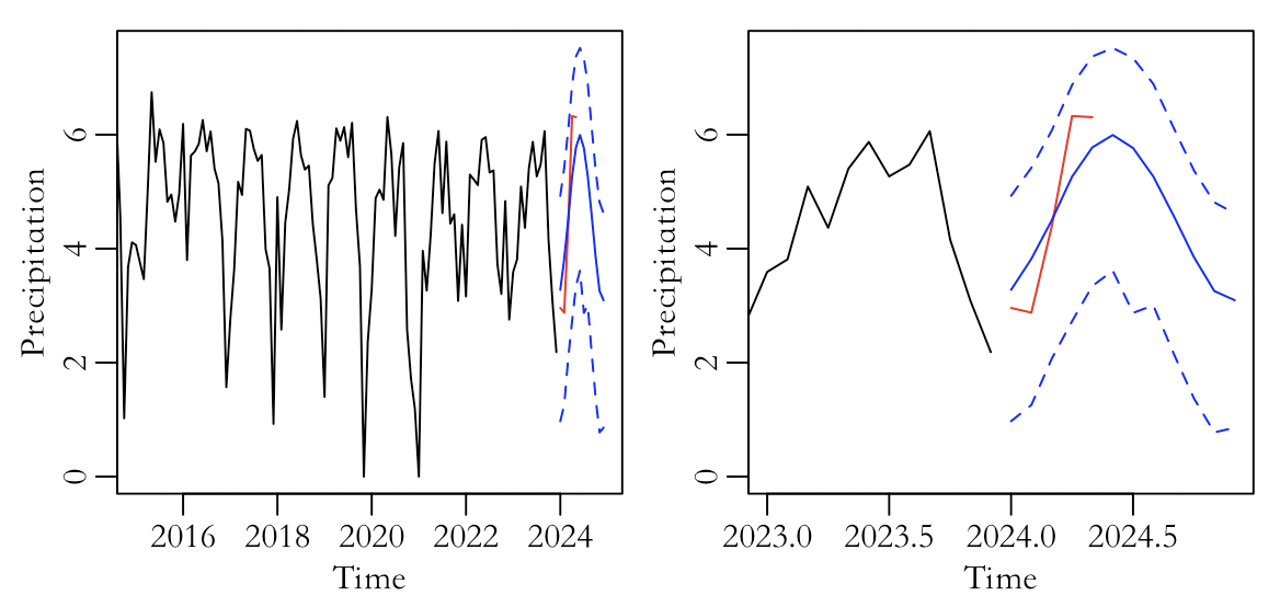
Figure 8: Time series graph under full-bootstrap with the latest data and predicted mean, along with upper and lower bounds (left) and details of the left graph (right).

Table 3: Coefficients of the newly fitted regression model under full bootstrap.

4. Conclusion

The convergence of escalating urban populations and the persistent peril of climate change underscores a heightened societal vulnerability to the impacts of extreme precipitation events [9]. This article models and fits the precipitation in Guangzhou from 2006 to 2023 using classical ARIMA and regression function models, and predicts the precipitation for the next year using Basic bootstrap and Full bootstrap prediction methods. To aid in the planning of effective flood mitigation infrastructure, it is paramount to conduct an exhaustive examination of the temporal patterns and spatial correlations associated with extreme precipitation occurrences [10]. The aim is to provide effective information for relevant government departments to plan.

In the model selection stage, the ACF plot of the first-order seasonal difference sequence shows a first-order integer order truncation. After applying the classical ARIMA model of ARIMA (0,0,0) (0,1,1) (12) to this sequence, the residual test result of the sequence is white noise, so the model is determined as ARIMA (0,0,0) (0,1,1) (12). During the modeling process, there was a situation where the first-order seasonal difference occurred, and in the subsequent final model coefficient estimation results, it was found that the value of the MA coefficient b1 was close to -1, indicating a problem of parameter approximate cancellation. Consideration may be due to the model setting: the coefficient of the moving average term approaching -1 may indicate that the seasonal effects in the data are very strong and close to cyclical reversals. But this may also be a signal of overfitting in the model, as such extreme values are not commonly seen in real data.

In the ARIMA model's prediction results, the Full bootstrap model's prediction results are closer to the true values based on the actual situation, and the prediction results are slightly better than the Basic bootstrap model. However, both methods have the problem of prediction interval bias, resulting in underestimation during the month of heavy rainfall in April. Considering that the MA coefficient is close to -1, it may lead to very unstable predicted values, and small errors may cause significant fluctuations in the predicted results. Therefore, the classical ARIMA model has poor fitting performance.

The ARMA model of regression function and residuals is known to have seasonality according to the previous analysis. The regression function directly extracts the seasonal components of the sequence, and the residual sequence without seasonality is directly modeled using ARMA. The residual of the sequence extracted by the regression function in this article is white noise, so there is no residual ARMA modeling. The explanatory variables of the regression function were ultimately reduced from 7 to 1 based on significance. The prediction process also adopts two methods: Basic bootstrap and Full bootstrap. Compared with the classical ARIMA model, the regression model's predictions are more accurate, and the true values fall within the prediction interval. The lower bound range in Full bootstrap prediction is smaller and more accurate.

References

[1]. Lan,Y., Shan D. (2024). Analysis of Rainstorm Disasters and Research on Urban Flood Prevention and Disaster Relief Strategies. Yellow River Water Conservancy Committee Shandong Yellow River Administration Bureau; Jinan Yellow River Administration Bureau Zhangqiu Yellow River Administration Bureau, 3.
[2]. Hongtao,L. (2014). Research on Combined Models for Rainfall Prediction in Irrigation Areas. Northeast Agricultural University.
[3]. Rezaiy,R., Shabri,A. (2024. )An innovative hybrid W-EEMD-ARIMA model for drought forecasting using the standardized precipitation index. Natural Hazards,1-30.
[4]. Cheng Maolin. (2015). Regression Prediction Model and Application Based on the Growth Curve of Trigonometric Functions [J]. Journal of Suzhou University of Science and Technology (Natural Science Edition), 32(04): 4-8.
[5]. Doko T., Firmin, Qazi H. (2023). On bootstrapping tests of equal forecast accuracy for nested models. Journal of Forecasting 42.7: 1844-1864.
[6]. Perera, I., Silvapulle, MJ. (2021). Bootstrap based probability forecasting in multiplicative error models. Journal of Econometrics 221.1: 1-24.
[7]. Tahyudin, I., Wahyudi,R., Nambo,H. (2022). SARIMA-LSTM combination for COVID-19 case modeling. IIUM Engineering Journal 23.2: 171-182.
[8]. Davino, C., Romano, R., Vistocco, D. (2022). Handling multicollinearity in quantile regression through the use of principal component regression. Metron, 80(2), 153-174.
[9]. Gimeno, L., Sorí, R., Vazquez, M., Stojanovic, M., Algarra, I., Eiras‐Barca, J., ... & Nieto, R. (2022). Extreme precipitation events. Wiley Interdisciplinary Reviews: Water, 9(6), e1611.
[10]. Yang, L., Franzke, C. L., & Duan, W. (2023). Evaluation and projections of extreme precipitation using a spatial extremes framework. International Journal of Climatology, 43(7), 3453-3475.
Cite this article
Yang,R. (2025). Temporal, Spatial Characteristics and Prediction of Precipitation in Guangzhou Based on the SARIMA Model. Theoretical and Natural Science,87,52-61.
Data availability
The datasets used and/or analyzed during the current study will be available from the authors upon reasonable request.
Disclaimer/Publisher's Note
The statements, opinions and data contained in all publications are solely those of the individual author(s) and contributor(s) and not of EWA Publishing and/or the editor(s). EWA Publishing and/or the editor(s) disclaim responsibility for any injury to people or property resulting from any ideas, methods, instructions or products referred to in the content.
About volume
Volume title: Proceedings of the 4th International Conference on Computing Innovation and Applied Physics
© 2024 by the author(s). Licensee EWA Publishing, Oxford, UK. This article is an open access article distributed under the terms and
conditions of the Creative Commons Attribution (CC BY) license. Authors who
publish this series agree to the following terms:
1. Authors retain copyright and grant the series right of first publication with the work simultaneously licensed under a Creative Commons
Attribution License that allows others to share the work with an acknowledgment of the work's authorship and initial publication in this
series.
2. Authors are able to enter into separate, additional contractual arrangements for the non-exclusive distribution of the series's published
version of the work (e.g., post it to an institutional repository or publish it in a book), with an acknowledgment of its initial
publication in this series.
3. Authors are permitted and encouraged to post their work online (e.g., in institutional repositories or on their website) prior to and
during the submission process, as it can lead to productive exchanges, as well as earlier and greater citation of published work (See
Open access policy for details).