1. Introduction

Combinational Equivalence Checking (CEC) [1-5] is a crucial process in digital circuit design, particularly in the verification of integrated circuits. As circuit designs become increasingly complex, ensuring that two versions of a circuit—typically a pre-optimized version and a post-optimized version—are functionally equivalent presents a significant challenge. CEC is employed to verify that these circuits produce identical outputs for all possible input combinations. This process is essential in design flows where design transformations, such as logic synthesis, optimization, or technology mapping, may alter the circuit’s structure but should not affect its functional behavior. The verification relies on various mathematical techniques, including Boolean algebra, Binary Decision Diagrams (BDDs), and satisfiability (SAT) solving, to efficiently determine the equivalence of large-scale designs. Consequently, CEC plays a pivotal role in maintaining the integrity and reliability of digital systems throughout the design lifecycle.

Functionally Reduced And-Inverter Graphs (FRAIGs) [6] are a data structure extensively used in CEC. FRAIGs represent Boolean functions as directed acyclic graphs, where nodes correspond to logical operations, specifically AND gates and inverters. The main advantage of FRAIGs lies in their ability to integrate structural hashing with functional reduction, allowing for the elimination of functionally equivalent nodes during the graph construction process. This results in a more compact representation, which reduces both memory usage and computational complexity. FRAIGs are particularly valuable for applications such as logic optimization, technology mapping, and equivalence checking, where efficient management of large circuits is critical. By incorporating simulation and SAT solving techniques, FRAIGs ensure that equivalent subgraphs are merged, thus minimizing redundancy. As a result, FRAIGs have become a fundamental tool in modern Electronic Design Automation (EDA) workflows, significantly enhancing the performance and scalability of circuit synthesis and verification processes.

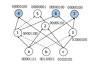
Figure 1: An example of equivalence nodes checking. Here, each node represents And gate and dash edge represents Not gate. The truth value of each node is the \( {2^{k}} \) -bit value of all different possible inputs value, here \( k \) is the number of prime inputs. For two nodes with same truth value, they are combinational equivalence. Here nodes \( 4,6,7 \) are equivalence nodes in blue.

Despite their advantages, FRAIGs present several challenges and limitations in the context of digital circuit synthesis and verification. A notable drawback is the potential increase in complexity during the graph construction process, especially for circuits with large fan-in or fan-out. Although FRAIGs are designed to reduce redundancy through functional reduction, the tasks of merging equivalent subgraphs and managing hash tables can introduce substantial computational overhead, particularly for very large designs. Moreover, FRAIGs may encounter difficulties when dealing with certain types of circuit transformations or optimizations that do not align well with the graph-based representation. For example, while FRAIGs are effective for standard logic optimizations, they may struggle with more complex transformations or dynamic changes in circuit structures. Additionally, the efficiency of FRAIGs can be affected by the trade-off between the granularity of functional reduction and the resulting graph size, where overly aggressive reduction may lead to a loss of structural information necessary for accurate equivalence checking. Therefore, addressing these challenges requires ongoing research and refinement to improve the scalability and applicability of FRAIGs across diverse design scenarios.

2. Problem Background

2.1. AIG and Subgraph

In this section, we first define And-Inverter graph, k-input fanout-free, and support nodes.

And-Inverter Graph. An And-Inverter Graph (AIG) [7] is a data structure to model combinational logic circuits. Let \( G=(V,E,PI,PO) \) be an AIG, where \( (V,E) \) is a directed acyclic graph, \( PI \) is the set of primary input vertices, and \( PO \) is the set of primary output vertices. Each vertex \( v∈V \) represents an And gate and \( v∈PI \) represents a primary input. Edges represent wires and can either be regular or complemented. For each vertex \( v∈V \) , \( FI(v) \) and \( FO(v) \) are the fanin and fanout vertices of \( v \) , i.e., in-neighbors and out-neighbors. For each vertex \( v∈V \) , \( |FI(v)|=2 \) , and for each primary input vertex \( v∈PI \) , \( |FI(v)|=0 \) .

K-Input Fanout-Free Subgraph.Given a set \( I \) of \( k \) input vertices , a \( k \) -input fanout-free subgraph \( G=(V,E,I,O) \) is also an AIG, where \( I \) are the input vertices and \( O⊂V \) are the output vertices. A fanout-free window should satisfy following fanout-free rules,

1. For each vertex \( v∈V\I \) , \( FI(v)⊂V \) .

2. For each vertex \( v∈V\O \) , \( FO(v)⊂V \) .

Support Nodes. Specifically, for any vertex \( v∈V\(O∪I) \) , its fanins and fanouts are also in the fanout-free subgraph. We call the vertices set fanout-free area. Roughly speaking, all vertices in a fanout-free window must be able to be fully expressed in the form of Boolean function by vertices of PI. Given \( k \) vertices \( I \) , the k-input maximum fanout-free subgraph is fully expanded by inputs \( I \) , whose fanout-free area is maximum.

Given a node \( v∈V \) in AIG \( G \) , a node \( s \) is called support node of \( v \) should satisfy,

3. \( s∈PI \) .

4. There exists a path from \( s \) to \( v \) in the AIG \( G \) .

For the set of all support nodes \( s∈S \) is called the support set of node \( v \) .

2.2. Equivalence Node Checking

Functional Equivalence Nodes. For each two nodes \( u,v∈V \) , the two nodes are called functional equivalence if for any input function, the value of nodes \( u \) and \( v \) keep equivalence.

Theorem 1. Equivalence node checking problem can be reduced to SAT satisfiability problem.

Proof 1. To check the equivalence of nodes \( {n_{1}} \) and \( {n_{2}} \) in an AIG, we can express the outputs of these nodes as Boolean functions. Construct a Boolean formula that captures the equivalence of the outputs. Let \( {F_{1}} \) and \( {F_{2}} \) represent the Boolean functions for the outputs of nodes \( {n_{1}} \) and \( {n_{2}} \) , respectively. Define a new Boolean formula:

\( F={F_{1}}⊕{F_{2}} \) (1)

where \( ⊕ \) denotes the XOR operation. The formula \( F \) is true if and only if \( {n_{1}} \) and \( {n_{2}} \) produce different outputs for some input combination. ◻

On the basis of Theorem 1, we can proof the NP-hardness of equivalence node checking and solve it by SAT-solver methods [8-10].

2.3. FRAIG

In this section, we discuss the traditional method Functionally Reduced AIG (FRAIG for short). The pseudocode presented in Algorithm 1 describes the process of reducing a Functionally Reduced And-Inverter Graph (FRAIG). The primary goal of this algorithm is to simplify the graph by merging nodes that are functionally equivalent, thereby minimizing redundancy while preserving the functional behavior of the original circuit.

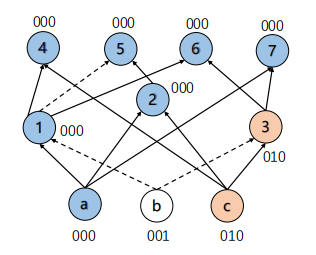
Figure 2: An example of FRAIG. Here, \( \lbrace 000,001,010\rbrace \) are the sample inputs of PI nodes. The blue nodes are same with \( 000 \) , and orange nodes are same as \( 010 \) in FRAIG method.

The algorithm takes as input an And-Inverter Graph (AIG) \( G \) and an integer \( k \) , which represents the number of random input samples by Monte Carlo. The output is a functionally reduced AIG, denoted by \( {G^{ \prime }} \) . The algorithm begins by initializing a hash table \( H \) and selecting \( k \) random input samples. The hash table \( H \) is used to store nodes from the graph \( G \) based on their truth values. In the first loop, each node \( v \) in \( G \) is processed and inserted into the hash table \( H \) such that nodes with the same truth values are grouped together in the same bucket. The second loop iterates over each bucket \( B \) in the hash table \( H \) . For every pair of nodes \( u \) and \( v \) within the same bucket, the algorithm checks whether the nodes are functionally equivalent using a SAT solver. If the SAT solver determines that the nodes are functionally equivalent, the nodes are merged in the output graph \( {G^{ \prime }} \) . Finally, the algorithm returns the reduced graph \( {G^{ \prime }} \) , which contains the minimized representation of the original circuit.

This approach leverages the efficiency of structural hashing and SAT solving to reduce the complexity of large circuits, making it particularly useful in electronic design automation (EDA) workflows. The use of random sampling and functional reduction ensures that the resulting graph \( {G^{ \prime }} \) retains the necessary functional properties while minimizing unnecessary redundancy.

Figure 2 shows an example of FRAIG. First, the FRAIG samples \( \lbrace 000,001,010\rbrace \) as the input of PI nodes \( a,b,c \) . After that, we can calculate the truth value of all nodes, as that nodes \( a,1,2,4,5,6,7 \) are same as \( 000 \) , and nodes \( c,3 \) are same as \( 010 \) . It takes \( C_{7}^{2}=21 \) times SAT-solver to check the equivalence of nodes with \( 000 \) , and \( C_{2}^{2}=1 \) times to check \( 010 \) value. So, it totally takes \( 22 \) times of SAT-solver.

3. Improved Sampling Methods

3.1. Sampling Improvement

To further improve the effectiveness of FRAIG in sampling, we propose a new algorithm shown in Algorithm 2. It is a method for the functional reduction of an And-Inverter Graph (AIG) \( G \) by identifying and merging nodes with equivalent functionality. The algorithm starts by initializing a hash table \( H \) and selecting a random sample of \( k \) input vectors. Each node \( v \) in \( G \) is processed by computing its truth value, after which it is inserted into the hash table \( H \) such that nodes with identical truth values are grouped together into buckets. The bucket \( {B_{0}} \) , which contains nodes with an all-zero truth value, is then specifically examined. For each node \( v \) in \( {B_{0}} \) , a SAT solver is employed to determine whether \( v \) can produce a non-zero output under any input condition. If the SAT solver returns True, indicating the existence of such inputs, these inputs are added to the sample input list, thus refining the input space and allowing for a more accurate assessment of node equivalence in subsequent steps. The algorithm proceeds by re-sampling the truth values based on this updated input space. For each bucket \( B \) in the hash table \( H \) , the algorithm compares pairs of nodes \( u \) and \( v \) within the bucket. The SAT solver is used to check if the XOR of their outputs \( u⊕v \) is unsatisfiable, which would indicate that \( u \) and \( v \) are functionally equivalent. If they are found to be equivalent, these nodes are merged in the reduced AIG \( {G^{ \prime }} \) . This process iteratively reduces the AIG by eliminating redundant nodes, leading to a more optimized representation. The algorithm concludes by returning the functionally reduced AIG \( {G^{ \prime }} \) , where equivalent nodes have been effectively merged, thereby optimizing the graph’s structure while maintaining its functional correctness.

Our Improved FRAIG method builds upon the standard FRAIG method by introducing several enhancements aimed at increasing the efficiency and accuracy of the functional reduction process. Both algorithms share the fundamental goal of reducing an And-Inverter Graph (AIG) by merging nodes that are functionally equivalent, thereby optimizing the graph’s structure. In the standard FRAIG approach, nodes are typically hashed based on their simulated values across a set of random input vectors, and equivalence is determined using SAT solvers. The FRAIG algorithm focuses on identifying and merging nodes that consistently produce identical outputs across these inputs, relying heavily on simulation and SAT solving techniques. The "Improved FRAIG" algorithm refines this process by incorporating a re-sampling step, which dynamically adjusts the set of input vectors based on the outcomes of SAT solver checks. This step is particularly crucial in ensuring that the input space is adequately explored, thereby reducing the likelihood of missing functionally equivalent nodes. Additionally, the "Improved FRAIG" algorithm explicitly processes nodes with an all-zero truth value by using a SAT solver to identify non-trivial cases where these nodes can produce non-zero outputs. By refining the input vector set and more thoroughly exploring node equivalences, the "Improved FRAIG" algorithm offers a more robust and precise reduction process, potentially leading to a more optimized AIG with fewer redundant nodes compared to the standard FRAIG approach.

3.2. Tree-like Nodes and Recoverage Nodes

In the optimization and verification of And-Inverter Graphs (AIGs), tree-like nodes and recoverage nodes exhibit distinct behaviors when processed by a SAT solver. Tree-like nodes are characterized by their simple, acyclic structure, where each node has a unique path from the root to the leaves. This simplicity allows SAT solvers to efficiently determine the functional equivalence or redundancy of tree-like nodes, as the absence of cycles reduces the complexity of the logic to be evaluated. Specifically, SAT solvers can quickly verify whether two tree-like nodes are functionally equivalent by comparing their outputs directly, leveraging the fact that their logical structure does not involve shared subgraphs or feedback loops.

On the other hand, recoverage nodes typically arise in more complex AIG structures, often involving shared subgraphs, multiple connections, or cycles. These nodes are encountered when certain nodes need to be revisited or reevaluated after optimization operations, such as node merging or functional simplification, have been applied. The complexity of recoverage nodes poses a greater challenge for SAT solvers, as these nodes may require a more thorough exploration of the logical space to ensure functional correctness. In particular, SAT solvers must handle the potential reintroduction of logic that was previously optimized away, necessitating the solver to perform additional iterations and potentially employ advanced techniques such as conflict analysis and learning to verify the accuracy of the recovered logic.

In summary, tree-like nodes allow for straightforward SAT solver processing due to their simple, acyclic nature, resulting in lower computational complexity. Conversely, recoverage nodes require more intricate handling by the SAT solver, as they involve complex logical structures that may necessitate re-sampling and more intensive verification to maintain the integrity of the AIG during optimization.

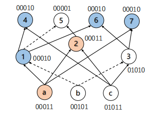
Figure 3: An example of our sampling method.

Figure 3 shows an example of our sampling method. After the results of random sampling of FRAIG shown in Figure 2, we calculate the inputs \( \lbrace 11,01,11\rbrace \) for PIs \( a,b,c \) that makes nodes \( a,1,2,4,5,6,7 \) are \( 1 \) . Note that only nodes \( 5 \) and \( 6 \) need SAT-solver because their recoverage structure. Other nodes are tree-like structure which could efficiently get the truth value. After that, our sampling method could detect nodes \( 1,4,6,7 \) with truth value \( 00010 \) and nodes \( a,2 \) with truth value \( 00011 \) . It takes \( C_{4}^{2}=6 \) times of SAT-solver to check the equivalence with truth value \( 00010 \) and \( 1 \) time to check \( 00011 \) . Totally, our method takes \( 2+6+1=9 \) SAT-solver, which is less than FRAIG.

4. Graph Partition Methods

4.1. Prime Output Partition

Baseline PO partition. Algorithm 3 presents a method for partitioning an And-Inverter Graph (AIG) into subgraphs. The algorithm takes as input an AIG \( G \) and an integer \( P \) , which represents the number of partitions. The goal of the algorithm is to generate a set of subgraphs \( S \) by dividing the primary outputs (POs) of the AIG into approximately equal-sized partitions.

The algorithm begins by calculating the number of primary outputs \( k \) that should be included in each partition. This value is computed as \( k=\frac{|PO|}{P} \) , where \( |PO| \) denotes the total number of primary outputs in the AIG.

Next, the algorithm iteratively constructs each subgraph. For each iteration \( i \) from 1 to \( P \) , the following steps are performed:

5. A random set of \( k \) primary output nodes \( O \) is selected from the remaining primary outputs.

6. The selected nodes \( O \) are then removed from the set of primary outputs to avoid duplication in future iterations.

7. The nodes in \( O \) are added to a new subgraph \( {W_{i}} \) .

8. The subgraph \( {W_{i}} \) is constructed by performing a Breadth-First Search (BFS) starting from the nodes in \( O \) , expanding to include all reachable nodes in the subgraph.

9. The constructed subgraph \( {W_{i}} \) is added to the set of subgraphs \( S \) .

After all \( P \) iterations are completed, the algorithm returns the set of subgraphs \( S \) .

The key idea behind this algorithm is to ensure that each partition contains a balanced number of primary outputs while leveraging BFS to construct the corresponding subgraphs. The use of random selection ensures that the partitioning is not biased, providing a baseline approach for further partitioning techniques. The removal of nodes from the primary output set after selection ensures that each node is only included in one partition, maintaining the disjoint nature of the subgraphs. The BFS step guarantees that each subgraph is fully connected and includes all nodes that are functionally related to the primary outputs in the partition.

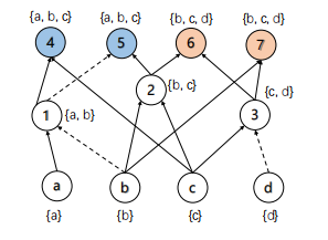
Figure 4: An example of support based partition. For the prime output nodes, \( 4,5 \) have same support nodes \( \lbrace a,b,c\rbrace \) and \( 6,7 \) have same support nodes \( \lbrace b,c,d\rbrace \) . So, our method could partition the graph into two subgraphs \( {G_{1}}=\lbrace a,b,c,1,2,4,5\rbrace \) and \( {G_{2}}=\lbrace b,c,d,2,3,6,7\rbrace \) .

Support based clustering. To further improve the efficiency and effectiveness of PO partition, we propose a support set based cluster method shown in Algorithm 4. It clusters output nodes in the AIG \( G \) based on the similarity of their support sets. The input to this algorithm is an AIG \( G \) , a specific output node \( {O_{i}} \) , and an integer \( k \) , which specifies the number of output nodes to be clustered together.

For each output node \( {O_{j}} \) in the set of primary outputs (PO), the algorithm calculates the similarity between the support sets of \( {O_{i}} \) and \( {O_{j}} \) . The similarity is defined as the ratio of the size of the intersection of the support sets to the size of their union:

\( Sim({O_{i}},{O_{j}})=\frac{|sup({O_{i}})∩sup({O_{j}})|}{|sup({O_{i}})∪sup({O_{j}})|}. \) (2)

Once the similarity scores are computed, the algorithm sorts all the output nodes by similarity to \( {O_{i}} \) and selects the top \( k-1 \) most similar output nodes to form a cluster with \( {O_{i}} \) . The algorithm then returns this set of clustered output nodes.

This approach is particularly useful in large-scale AIGs where managing complexity through partitioning can significantly reduce computational overhead in subsequent processing tasks, such as SAT-solving or equivalence checking.

4.2. K-input Subgraph Partition

K-input support calculation.Algorithm 5 computes the support set for each vertex in an And-Inverter Graph (AIG) \( G \) and identifies the nodes that have support sets larger than a given threshold \( B \) . The input to the algorithm is an AIG \( G \) and an integer \( B \) , which represents the maximum allowable size of a support set.

The algorithm begins by initializing an empty set \( S \) , which will store nodes whose support sets exceed the threshold \( B \) . For each vertex \( v \) in the AIG, processed in topological order, the algorithm determines the support set of \( v \) based on its fan-in nodes. If \( v \) is a primary input (PI), its support set is simply \( \lbrace v\rbrace \) . For non-PI vertices, the support set \( sup(v) \) is calculated by taking the union of the support sets of its fan-in nodes \( F{I_{1}}(v) \) and \( F{I_{2}}(v) \) . If either fan-in node is already in set \( S \) , indicating that its support set exceeded the threshold \( B \) , the support set for that node is limited to just itself, to prevent further growth of support sets.

If the size of the support set \( sup(v) \) exceeds \( B \) , vertex \( v \) is added to set \( S \) . The algorithm continues this process for all vertices in the graph. Finally, the algorithm returns the support sets for all vertices, along with the set \( S \) of nodes whose support sets exceeded the threshold.

K-input subgraph partition.Algorithm 6 partitions an And-Inverter Graph (AIG) \( G \) into a set of subgraphs based on the results from the \( k \) -input support calculation. The input to the algorithm is the AIG \( G \) and an integer \( B \) , which is the threshold for the support set size.

The algorithm begins by calculating the \( k \) -input supports for all vertices using the previously defined \( k \) -input support calculation algorithm (Algorithm), resulting in a set \( S \) of vertices whose support sets exceed the threshold. The set of primary outputs (POs) is then updated to include the vertices in \( S \) , resulting in an augmented set \( P{O^{ \prime }} \) .

Next, the algorithm applies a clustering algorithm (Algorithm 4) to partition the graph based on the updated set \( P{O^{ \prime }} \) . The goal is to create subgraphs that are more manageable and can be processed independently. Finally, the algorithm returns the set of partitioned subgraphs.

This algorithm partitions an AIG into subgraphs based on the \( k \) -input support sets calculated in the previous algorithm. By including the vertices with large support sets in the set of primary outputs, the algorithm ensures that the resulting subgraphs are well-formed and suitable for further processing.

5. Experiment

We implement our method in C++ using ABC library [11] and EPFL logic synthesis benchmark [12]. We select four relatively small circuits and seven large circuits from EPFL benchmarks [12] to present the scalability of our algorithms. The details of datasets are shown in Table 1. All experiments have been conducted on an Intel(r) Core(tm) i7-12700k processor with 32 GB RAM. We mark the running time as infinite, denoted as ‘-’ if the algorithm runs exceeding 3 hours.

Table 1: Comparison of FRAIG and our sampling method on small AIGs.

Effective and efficiency of FRAIG and our sampling method. The experimental results presented in Table 1 compare the performance of the traditional FRAIG method with our proposed sampling method on small And-Inverter Graphs (AIGs). The comparison focuses on two key metrics: the number of SAT-solver calls (# SAT) and the computation time (in seconds).

For the dataset "cavlc," the FRAIG method requires 499 SAT-solver calls, taking a total of 0.49 seconds to complete the process. In contrast, our sampling method significantly reduces the number of SAT-solver calls to just 27 and completes in a much shorter time of 0.06 seconds. This trend of improved performance with our sampling method is consistent across all datasets. For instance, in the "ctrl" dataset, FRAIG uses 79 SAT-solver calls in 0.10 seconds, whereas our sampling method only requires 15 SAT-solver calls and completes in 0.01 seconds. Similarly, for the "dec" dataset, FRAIG requires 186 SAT-solver calls, consuming 0.13 seconds, compared to just 11 SAT-solver calls and 0.01 seconds with our method. Finally, in the "int2float" dataset, FRAIG makes 244 SAT-solver calls in 0.15 seconds, while our sampling approach requires only 23 calls and finishes in 0.01 seconds.

Overall, the results demonstrate that our sampling method consistently outperforms the traditional FRAIG approach across all tested datasets, reducing both the number of SAT-solver calls and the computation time. This indicates that our method is more efficient and scalable, particularly for handling small AIGs, where the reduction in SAT-solver calls directly translates to faster execution times.

Table 2: Comparison of Strash and our 6-input Subgraph Partition

Table 3: Comparison of FRAIG and our \( \frac{|PI|}{2} \) -input Subgraph Partition

The experimental results shown in Tables 2 and 3 compare the performance of different graph partitioning and reduction methods: the Strash method versus the \( 6 \) -input Subgraph Partition and the FRAIG method versus the \( \frac{n}{2} \) -input Subgraph Partition, respectively. The comparison is based on three metrics: the number of nodes reduced by the algorithm (# RDC), computation time (in seconds), and the efficiency of node reduction per unit time ( \( \frac{\ \ \ RDC}{Time} \) ).

Table 2 illustrates the comparison between Strash and the \( 6 \) -input Subgraph Partition. The \( 6 \) -input Subgraph Partition consistently outperforms the Strash method across all datasets. For instance, in the "div" dataset, Strash does not achieve any node reduction (0 RDC in 0.01 seconds), whereas the \( 6 \) -input Subgraph Partition reduces 849 nodes in 0.96 seconds, resulting in an efficiency of 883.85. This trend is observed across other datasets such as "hyp," "log2," "multiplier," "sixteen," "twenty," and "twentytr," where the \( 6 \) -input Subgraph Partition method significantly increases the number of reduced nodes and maintains higher efficiency scores. For example, for the "twenty" dataset, the \( 6 \) -input Subgraph Partition method reduces 39,408 nodes in 78.63 seconds, achieving an efficiency of 501.18, while Strash only reduces 23 nodes in 4.91 seconds with a much lower efficiency of 4.68.

Table 3 compares the FRAIG method with the \( \frac{|PI|}{2} \) -input Subgraph Partition method. The \( \frac{|PI|}{2} \) -input Subgraph Partition method demonstrates superior performance in terms of node reduction and efficiency. For example, in the "div" dataset, FRAIG reduces 15,933 nodes in 51.99 seconds with an efficiency of 306.46. In contrast, the \( \frac{|PI|}{2} \) -input Subgraph Partition method reduces 11,991 nodes in only 3.32 seconds, resulting in a significantly higher efficiency of 3611.75. Similar improvements are observed in other datasets such as "hyp," "log2," and "multiplier," where the \( \frac{|PI|}{2} \) -input Subgraph Partition method consistently reduces more nodes in less time or achieves higher efficiency. Notably, for more complex datasets like "sixteen," "twenty," and "twentytr," FRAIG fails to produce results (indicated by "-") in limited time, while the \( \frac{|PI|}{2} \) -input Subgraph Partition method demonstrates robust performance, reducing millions of nodes with efficiencies of 796.76, 802.72, and 639.35, respectively.

In summary, the results indicate that both the \( 6 \) -input and \( \frac{|PI|}{2} \) -input Subgraph Partition methods significantly outperform their respective baselines (Strash and FRAIG) in terms of node reduction capabilities and computational efficiency across a variety of datasets, especially for larger and more complex graph structures. This demonstrates the effectiveness of the proposed subgraph partitioning strategies in optimizing graph reduction processes.

6. Conclusion and Future Work

In this paper, we have presented novel approaches to enhance the efficiency and accuracy of combinational equivalence checking using Functionally Reduced And-Inverter Graphs (FRAIGs). Our proposed methods, including improved sampling techniques and advanced graph partitioning strategies, have shown to significantly reduce computational complexity and improve the scalability of equivalence checking in large and complex circuits. By leveraging support node analysis and probability distribution modeling, we effectively reduced redundancy and enhanced the performance of the equivalence identification process. Future work will focus on further optimizing these techniques and exploring new algorithms to handle increasingly complex digital circuit designs.

There also exist some direction to extend this paper in the future work. First, we could try to set different parameters of \( P \) and \( B \) for different datasets to get the more effective solution. Second, we could try to sampling a better initial input for FRAIG based on the probability distribution of different datasets to reduce the times of SAT-solver.

References

[1]. L. Amar´u, F. Marranghello, E. Testa, C. Casares, V. Possani, J. Luo, P. Vuillod, A. Mishchenko, and G. De Micheli. Sat-sweeping enhanced for logic synthesis. In 2020 57th ACM/IEEE Design Automation Conference (DAC), pages 1–6. IEEE, 2020.
[2]. M. Backes, J. M. Matos, R. Ribas, and A. Reis. Reviewing aig equivalence checking approaches. In Proceedings of the ACM Microelectronics Student Forum, pages 1–4, 2014.
[3]. S. Chatterjee and N. Een. Improvements to combinational equivalence checking.
[4]. A. Mishchenko, S. Chatterjee, R. Brayton, and N. Een. Improvements to combinational equivalence checking. In Proceedings of the 2006 IEEE/ACM international conference on Computer-aided design, pages 836–843, 2006.
[5]. Q. Zhu, N. Kitchen, A. Kuehlmann, and A. Sangiovanni-Vincentelli. Sat sweeping with local observability don’t-cares. In Proceedings of the 43rd Annual Design Automation Conference, pages 229–234, 2006.
[6]. A. Mishchenko, S. Chatterjee, R. Jiang, and R. K. Brayton. Fraigs: A unifying representation for logic synthesis and verification. Technical report, ERL Technical Report, 2005.
[7]. C. Yu, M. Ciesielski, and A. Mishchenko. Fast algebraic rewriting based on and-inverter graphs. IEEE Transactions on Computer-Aided Design of Integrated Circuits and Systems, 37(9):1907–1911, 2017.
[8]. N. E´en and N. S¨orensson. An extensible sat-solver. In International conference on theory and applications of satisfiability testing, pages 502–518. Springer, 2003.
[9]. W. Gong and X. Zhou. A survey of sat solver. In AIP Conference Proceedings, volume 1836. AIP Publishing, 2017.
[10]. Y. Hamadi, S. Jabbour, and L. Sais. Manysat: a parallelsat solver. Journal on Satisfiability, Boolean Modeling and Computation, 6(4):245–262, 2010.
[11]. R. Brayton and A. Mishchenko. Abc: An academic industrial-strength verification tool. In International Conference on Computer Aided Verification, pages 24–40, 2010.
[12]. L. Amar´u, P.-E. Gaillardon, and G. De Micheli. The epfl combinational benchmark suite. In Proceedings of the 24th International Workshop on Logic & Synthesis (IWLS), 2015.
Cite this article
Tang,L. (2025). Combinational Equivalence Checking on AIGs. Theoretical and Natural Science,87,91-102.
Data availability
The datasets used and/or analyzed during the current study will be available from the authors upon reasonable request.
Disclaimer/Publisher's Note
The statements, opinions and data contained in all publications are solely those of the individual author(s) and contributor(s) and not of EWA Publishing and/or the editor(s). EWA Publishing and/or the editor(s) disclaim responsibility for any injury to people or property resulting from any ideas, methods, instructions or products referred to in the content.
About volume
Volume title: Proceedings of the 4th International Conference on Computing Innovation and Applied Physics
© 2024 by the author(s). Licensee EWA Publishing, Oxford, UK. This article is an open access article distributed under the terms and
conditions of the Creative Commons Attribution (CC BY) license. Authors who
publish this series agree to the following terms:
1. Authors retain copyright and grant the series right of first publication with the work simultaneously licensed under a Creative Commons
Attribution License that allows others to share the work with an acknowledgment of the work's authorship and initial publication in this
series.
2. Authors are able to enter into separate, additional contractual arrangements for the non-exclusive distribution of the series's published
version of the work (e.g., post it to an institutional repository or publish it in a book), with an acknowledgment of its initial
publication in this series.
3. Authors are permitted and encouraged to post their work online (e.g., in institutional repositories or on their website) prior to and
during the submission process, as it can lead to productive exchanges, as well as earlier and greater citation of published work (See
Open access policy for details).