1. Introduction

Partial differential equations (PDEs) are a central mathematical tool for modeling and analyzing various phenomena in fields such as physics, engineering, biology, and economics. These equations describe relationships involving unknown functions of multiple variables and their partial derivatives. Many physical processes, such as heat diffusion, fluid mechanics, and electromagnetic wave propagation, are governed by PDEs. Finding solutions to these equations, either analytically or numerically, is critical for understanding the behavior of complex systems and predicting their evolution.

The variational formulation is a powerful tool for PDEs, especially in the context of physics and engineering problems. Generally, by using test functions and Green’s formulas, the equation can be transformed into the related variational formulation. Then, the well-posedness of the variational formulation can be proven by applying the Lax-Milgram theorem and related theories. One can see more concepts and theories related to Green’s formulas, Sobolev spaces and the Lax-Milgram theorem in reference[2-7].

We are interested in some problems arising in the study of electromagnetic wave propagation in the presence of metals or certain types of metamaterials after referencing several papers and books ([8-10]), and a detailed description of the background of this problem can be found in . Roughly speaking, variations in the electromagnetic field within a material or metamaterials are governed by Maxwell’s equations, which involve physical coefficients like dielectric permittivity \( ε \) and \( μ \) magnetic permeability \( μ \) and cause these coefficients to become negative.

In fact, studying Maxwell’s equations in media combining positive and negative materials raises unique challenges. The sign-changing parameters lead to PDEs that do not fit into the standard frameworks, and the Lax-Milgram cannot be applied directly in this case since we lack the coercivity. We classify such problems as non-coercive problems.

In this paper, we apply the T-isomorphism method to analyze these problems, also introduced in [1]. More specifically, we study Poisson-type equations that are formally the same as in [1], but in fully asymmetric configurations, which is a fundamental difference from the study in [1]. In fully asymmetric configurations, it is not possible to use a similar method as in [1] to construct the isomorphism T, which requires us to construct a completely different isomorphism T to solve these problems. In conclusion, we obtain the well-posedness of these problems under some parameters and asymmetric parameters that are related.

2. Preliminaries

In this paper, \( Ω \) is assumed to be a bounded domain with a regular boundary. The outward unit normal vector on \( ∂Ω \) is denoted by \( n=({n_{i}}) \) , and the Lebesgue measures in \( Ω \) and on \( ∂Ω \) are represented by \( dx \) and \( ds \) , respectively.

2.1. Hilbert Space

In this subsection, we introduce the Hilbert space. Firstly, we give the definitions of the linear form and bilinear form.

Definition 2.1. A linear form \( L \) on a real vector space \( V \) is a function that takes a single variable from the vector space \( V \) and maps it to a real number, while satisfying specific properties for any scalar \( k \) and any vectors \( u \) and \( v \) , as described by the following equations. \( \begin{matrix}L(lv) & =lL(v), \\ L(u+v) & =L(u)+L(v). \\ \end{matrix} \)

Definition 2.2. A bilinear form \( b \) on a real vector space \( V \) is a function that takes two variables from \( V×V \) and maps them to a real number, which satisfies certain properties for any scalar \( l \) and any vectors \( u,v,{u_{1}},{u_{2}},{v_{1}},{v_{2}} \) , \( \begin{matrix}b(lu,v) & =b(u,lv)=lb(u,v), \\ b({u_{1}}+{u_{2}},v) & =b({u_{1}},v)+b({u_{2}},v), \\ b(u,{v_{1}}+{v_{2}}) & =b(u,{v_{1}})+b(u,{v_{2}}). \\ \end{matrix} \)

Based on the definition of bilinear form, we can introduce the following definition of inner product space.

Definition 2.3. A real inner product space is a real vector space equipped with an inner product. The inner product is a bilinear form \( ⟨\cdot ,\cdot ⟩:V×V→R \) that satisfies the following properties: \( \begin{matrix} & ⟨u,v⟩=⟨v,u⟩ for allu,v∈V; \\ & ⟨v,v⟩≥0 for allv∈V; \\ & ⟨v,v⟩=0if and only ifv=0. \\ \end{matrix} \)

Then we introduce the following definition of Hilbert space.

Definition 2.4. We define a real Hibert space as a complete real inner product space on \( V \) , with a scaler product which is noted as \( ⟨a,b⟩ \) . More precisely, it is complete for the norm associated to this scalar product, which is \( ∥a{∥_{V}}=\sqrt[]{⟨a,a{⟩_{V}}},for alla∈V. \)

2.2. Sobolev Space

We give following the definition of the Sobolev space \( {H^{n}} \) , where \( n∈{N^{+}} \) .

Remark 2.5. Let \( Ω \) be an open set of \( {R^{N}} \) . Then we are able to define the Sobolev space \( {H^{1}}(Ω) \) by

\( {H^{1}}(Ω)=\lbrace v∈{L^{2}}(Ω) | \frac{∂v}{∂{x_{i}}}∈{L^{2}}(Ω)for alli∈\lbrace 1,…,N\rbrace \rbrace \)

where \( \frac{∂v}{∂{x_{i}}} \) is the ith weak partial derivative of \( v \) . To generalize, we further define \( {H^{n}}(Ω) (n≥2) \) by

\( {H^{n}}(Ω)=\lbrace v∈{L^{2}}(Ω)such that{∂^{α}}v∈{L^{2}}(Ω)for allαwith|α|≤n\rbrace \)

with

\( {∂^{α}}v(x)=\frac{{∂^{|α|}}v}{∂x_{1}^{{α_{1}}}⋯∂x_{N}^{{α_{N}}}}(x), \)

where \( {∂^{α}}v \) is taken in the weak sense. Here \( α=({α_{1}},…,{α_{N}}) \) is multi-index with \( {α_{i}}≥0 \) and \( |α|=\sum _{i=1}^{N}{α_{i}} \) . Moreover,the inner product is written as \( \begin{matrix}⟨u,v⟩=\int _{Ω}^{​}(u(x)v(x)+∇u(x)\cdot ∇v(x))dx. \\ \end{matrix} \) Meanwhile, the norm is given in following form \( \begin{matrix}∥v{∥_{{H^{1}}(Ω)}}=(\int _{Ω}^{​}{(({|v(x)|^{2}}+{|∇v(x)|^{2}})dx)^{\frac{1}{2}}} \\ \end{matrix} \)

After discussing the general case of \( {H^{1}}(Ω) \) , we start to introduce a specific subspace of \( {H^{1}}(Ω) \) , noted as \( H_{0}^{1}(Ω) \) .

Definition 2.6. Let \( Ω \) be a bounded region domain. The Sobolev space \( H_{0}^{1}(Ω) \) is defined as the closure of the space of functions \( C_{c}^{∞}(Ω) \) , which are of class \( {C^{∞}}(Ω) \) and have compact support in \( Ω \) , in the function space \( {H^{1}}(Ω) \) . \( H_{0}^{1}(Ω) \) is actually the subspace of \( {H^{1}}(Ω) \) which consists of functions that cancel on the edge \( ∂Ω \) where \( ∂Ω \) is equal to \( 0 \) for functions of \( C_{c}^{∞}(Ω) \) .

Remark 2.7. Since \( H_{0}^{1}(Ω) \) is a closed subspace of \( {H^{1}}(Ω) \) , \( H_{0}^{1}(Ω) \) is also a Hilbert space.

Proposition 2.8. (Poincaré inequality) Let \( Ω \) be a regular bounded open set of \( {C^{1}} \) . There exists a constant \( C≥0 \) such that, for any function \( v∈H_{0}^{1}(Ω) \) , \( \int _{Ω}^{​}{|v(x)|^{2}}dx≤C\int _{Ω}^{​}{|∇v(x)|^{2}}dx \)

After discussing the definition and properties of Sobelev space \( H_{0}^{1}(Ω) \) , we will move on to investigating the equivalent norm.

Definition 2.9. Let X be a normed vector space. Two norms are equivalent if they both can be controlled by another norm. Specifically, the norms \( ∥\cdot {∥_{α}} \) and \( ∥\cdot {∥_{β}} \) are considered equivalent if there exist \( a,b∈{R_{+}} \) , such that for any \( x∈X \) , we have \( \begin{matrix}a∥x{∥_{α}}≤∥x{∥_{β}}≤b∥x{∥_{α}}. \\ \end{matrix} \)

Combine Definition 2.9 and Proposition 2.8, we can infer the following corollary.

Corollary 2.10. The norm of \( H_{0}^{1}(Ω) \) can be also defined as \( ∥v{∥_{H_{0}^{1}(Ω)}}:={(\int _{Ω}^{​}{|∇v(x)|^{2}}dx)^{\frac{1}{2}}}=∥∇v{∥_{{L^{2}}(Ω)}}. \)

Then we move on to the introduction of the Rellich–Kondrachov theorem.

Theorem 2.11. (Rellich–Kondrachov Theorem) For any bounded sequence in \( {H^{1}}(Ω) \) , we can extract a sub-sequence that converges in \( {L^{2}}(Ω) \) .

Then we introduce the following Green’s formulae, which are also regarded as integration by parts in high-dimensional spaces.

Theorem 2.12. (Green’s formulae) If \( u,w∈{H^{1}}(Ω) \) , then we have \( \int _{Ω}^{​}u\frac{∂w}{∂{x_{i}}}dx=-\int _{Ω}^{​}\frac{∂u}{∂{x_{i}}}wdx+\int _{∂Ω}^{​}uw{n_{i}}ds. \) Moreover, given \( u∈{H^{2}}(Ω) \) and \( w∈{H^{1}}(Ω) \) , we are able to derive \( \int _{Ω}^{​}Δuwdx=-\int _{Ω}^{​}∇u\cdot ∇wdx+\int _{∂Ω}^{​}\frac{∂u}{∂n}wds. \)

With all the above definitions and explanations of each theorem, we now introduce Lax-Milgram theorem.

2.3. Lax-Milgram Theorem

Some Poisson-type equations can be reformulated using equations (2.3) and (2.4) to derive their variational formulation. Lax-Milgram theorem is an essential tool for obtaining the well-posedness of a variational formula in a real Hilbert space, denoted as \( V \) . The well-posedness of a PDE’s variational formulation in a Hilbert space is generally equivalent to the well-posedness of the original PDE. We can analyze the given variational formulation’s well-posedness by utilizing the Lax-Milgram theorem.

We consider the following variational formulation:

\( Findu∈Vsuch thata(u,v)=L(v), ∀v∈V. \)

Before introducing Lax-Milgarm theorem, we need to give the assumptions of \( a(u,v) \) and \( L(v) \) , which are respectively

1. Bounded linear form. More precisely, there exists \( C \gt 0 \) such that

\( |L(v)|≤C∥v∥, ∀v∈V \)

2. Bounded bilinear form. More precisely, there exists \( C \gt 0 \) such that

\( |a(u,v)|≤C∥u{∥_{V}}∥v{∥_{V}}, ∀u,v∈V. \)

3. coercivity of the bilinear form. More precisely, there exists \( α \gt 0 \) such that

\( a(v,v)≥α∥v∥_{V}^{2}, ∀v∈V. \)

Theorem 2.13. (Lax-Milgram Theorem) Given \( V \) a real Hilbert space, If \( L(\cdot ) \) and \( a(\cdot ,\cdot ) \) satisfy (2.6), (2.7) and (2.8), then there is a unique solution to (2.5).

2.4. T-isomorphism approach

The Lax-Milgram theorem is very useful in the study of many Poisson-type equations, however, it cannot be applied directly to non-coercive problems. Non-coercive problems generally refer to issues in the variational formulation (2.2) where \( a(\cdot ,\cdot ) \) does not satisfy the condition (2.8). For non-coercive problems, we have another approach to analyse these problems, which we generally call the T-isomorphism approach. See also .

We then introduce the T-isomorphism approach.[9]

Theorem 2.14. Given \( V \) a real Hilbert space. If \( L(\cdot ) \) is a bounded linear form on \( V \) and \( a(\cdot ,\cdot ) \) is a bounded bilinear form on \( V \) . Also, we assume that there is an isomorphism \( T \) of \( V \) such that the bilinear form \( (u,v)↦a(u,Tv) \) is coercive on \( V×V \) , then there exists a unique solution to variational formuation (2.5) .

Proof. We refer to the proof of [10, Lemma 3.6].

3. Anaylsis of non-coercive problems

3.1. Maxwell’s equation in metamaterials

We aim to explore the well-posedness of a Maxwell equation tailored to a specific material. To accommodate this material type, we propose a generalized form of Maxwell’s equation. Consider a bounded and regular domain \( Ω⊂{R^{2}} \) . We partition \( Ω \) into two subdomains \( {Ω_{1}},{Ω_{2}}, \) such that \( \overline{Ω}={\overline{Ω}_{1}}∪{\overline{Ω}_{2}} \) and \( {Ω_{1}}∩{Ω_{2}}=∅. \) Currently, Maxwell’s equation is not able to describe the mixing of metamaterials on different subdomains, thereby we need the introduction of additional functions. Therefore, we assume

\( σ(x,y)=\begin{cases}\begin{matrix}{σ_{1}} & if(x,y)∈{Ω_{1}}, \\ {σ_{2}} & if(x,y)∈{Ω_{2}}. \\ \end{matrix}\end{cases} \)

In this case, \( {σ_{1}},{σ_{2}} \) are two constants where \( {σ_{1}} \gt 0 \) and \( {σ_{2}} \lt 0 \) . We are interested in studying the well-posedness of the resulting non-coercive problem.

\( Findu∈H{​^{1}}(Ω)such that -div(σ∇u)=f inΩ. \)

Here, \( f∈{L^{2}}(Ω) \) denotes the source term. We also introduce the following notation

\( \begin{matrix}κ=\frac{{σ_{2}}}{{σ_{1}}}. \\ \end{matrix} \)

Here \( κ \) is an essential indicator in the analysis section, which is crucial in the range of well-posedness. We will consider the well-posedness of (3.1) in two different domains. The choice of functions \( f \) and \( σ \) vary depending on the specific application of this equation. For more sophisticated models, we are interested in the wellposedness of a more general mathematical problem and so we introduce region of \( Ω \) . Let \( Ω \) be the bounded domain of \( {R^{2}} \) defined by

\( Ω=\lbrace (x,y)∈{R^{2}}such that-1 \lt x \lt 2n-1and0 \lt y \lt 1\rbrace . \)

Also, we have \( \overline{Ω}={\overline{Ω}_{1}}∪{\overline{Ω}_{2}} \) , and

\( \begin{matrix} & {Ω_{1}}=\lbrace (x,y)∈{R^{2}}such that-1 \lt x \lt 0and0 \lt y \lt 1\rbrace , \\ & {Ω_{2}}=\lbrace (x,y)∈{R^{2}}such that0 \lt x \lt 2n-1and0 \lt y \lt 1\rbrace . \\ \end{matrix} \)

And we will also introduce the boundaries of two frontiers of the region of leftest and rightest respectively, for which we define

\( {γ_{1}}=\lbrace -1\rbrace ×(0,1),{γ_{2}}=\lbrace 2n-1\rbrace ×(0,1). \)

Morever, We note \( Σ \) as the boundary between \( {Ω_{1}} \) and \( {Ω_{2}} \) , \( {Γ_{10}}=(-1,0)×(0,0)∪(-1,1)×(0,1) \) as the left upward and downward frontiers of the domain, and \( {Γ_{20}}=(0,0)×(2n-1,0)∪(0,1)×(2n-1,1) \) as the right upward and downward frontiers of the domain. To solve the problem, we divide the region into two domains, where

\( ∂{Ω_{1}}={γ_{1}}∪Σ∪{Γ_{10}}, ∂{Ω_{2}}={γ_{2}}∪Σ∪{Γ_{20}}, \)

and the boundaries of each domain is respectively

\( {Ω_{1}}=(-1,0)×(0,1), {Ω_{2}}=(0,2n-1)×(0,1). \)

Finally, we make the definition of the Hilbert subspace \( V \) of \( {H^{1}}(Ω) \) as follows for our further exploration of this analysis \( V={V_{per}} \) , where “per” stands for periodic. Given two real values \( {σ_{1}} \gt 0 \) and \( {σ_{2}} \lt 0 \) , let \( σ \) be the function defined almost everywhere in \( Ω \) by \( σ(x,y)={σ_{j}} \) in \( {Ω_{j}} \) for \( j=1,2 \) . Finally, we define the Hilbert subspace \( V \) of \( {H^{1}}(Ω) \) as follows

\( \begin{matrix}{V_{per}}:=\lbrace v∈{H^{1}}(Ω) | v=0on{Γ_{10}}∪{Γ_{20}}andv(-1,y)=v(2n-1,y)for ally∈(0,1)\rbrace \\ \end{matrix} \)

For our analysis, we consider the following variational formulation,

\( Findu∈Vsuch that a(u,v)=L(v), \)

where

\( \begin{matrix} & a(u,v)=σ\int _{Ω}^{​}∇u(x)\cdot ∇v(x)dx={σ_{1}}\int _{{Ω_{1}}}^{​}∇u(x)\cdot ∇v(x)dx+{σ_{2}}\int _{{Ω_{2}}}^{​}∇u(x)\cdot ∇v(x)dx,  \\ & L(v)=\int _{Ω}^{​}f(x)v(x)dx. \\ \end{matrix} \)

Remark 3.1. In fact, by applying the Rellich-Kondrachov Theorem 2.11, we can also deduce the Poincaré inequality (2.1) for all functions in \( {V_{per}} \) . So the norm of \( {V_{per}} \) can be defined as follows: \( \begin{matrix}∥v{∥_{{V_{per}}}}:={(\int _{Ω}^{​}{|∇v(x)|^{2}}dx)^{\frac{1}{2}}}=∥∇v{∥_{{L^{2}}(Ω)}}. \\ \end{matrix} \)

3.2. Summary of main results

Through our analysis of these two equations, we were able to reach several conclusions. The main results are presented below. We first resolve the case where both constants are positive, then present results for more sophisticated domains and boundary conditions. We conclude with a general result inspired by the Riesz representation theorem.

Theorem 3.2. Consider the case when \( n=1 \) , where \( Ω=(-1,1) \) . Specifically, we divide the region into \( {Ω_{1}}=(-1,0)×(0,1) \) and \( {Ω_{2}}=(0,1)×(0,1) \) . For this geometry, the variational formulation (3.2) admits a unique solution when \( κ≠-1 \) .

Theorem 3.3. Consider the case when \( n=2 \) , where \( Ω=(-1,3) \) . Specifically, we divide the region into \( {Ω_{1}}=(-1,0)×(0,1) \) and \( {Ω_{2}}=(0,3)×(0,1) \) . For this geometry, the variational formulation (3.2) admits a unique solution when \( κ∈(-∞,-3)∪(-\frac{1}{3},0) \) .

Theorem 3.4. Consider the generalized case when \( n∈Z \) , where \( Ω=(-1,2n-1) \) and we divide the region into \( {Ω_{1}}=(-1,0)×(0,1) \) and \( {Ω_{2}}=(0,2n-1)×(0,1) \) . For this geometry, the variational formulation (3.2) admits a unique solution when \( κ∈(-∞,1-2n)∪(-\frac{1}{2n-1},0) \) .

3.3. Proof of main results

3.4. Proof of Theorem 3.1

In fact, this case has been essentially proven in [1]. Since we have a symmetric configuration when \( n=1 \) , we can directly apply the same method as in [1,(3.6)] to construct an appropriate isomorphism \( T \) , and then we can follow the proof of [1] to show that the variational formulation (3.2) admits a unique solution when \( κ≠-1 \) .

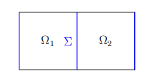
Figure 1: Configuration for case \( n=1 \)

3.5. Proof of Theorem 3.2

First of all, we construct \( {Ω_{1}} \) and \( {Ω_{2}} \) and divide \( {Ω_{2}} \) into several regions in the following subdomains

\( {Ω_{2}}=\begin{cases}\begin{matrix}{C_{1}}, & {C_{1}}∈(0,1)×(0,1), \\ {C_{2}}, & {C_{2}}∈(1,2)×(0,1), \\ {C_{3}}, & {C_{3}}∈(2,3)×(0,1). \\ \end{matrix}\end{cases} \)

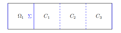
Figure 2: Configuration for case \( n=2 \)

To achieve the solution for solving the well-posedness of this case when \( n=2 \) , we ought to create a T-isomorphism and use the Lax-Milgram Theorem. We have to directly construct \( Tv(x,y) \) on \( Ω \) so that it is always continuous on \( {Ω_{2}} \) , which is denoted as follows:

\( Tv(x,y)=\begin{cases}\begin{matrix}v(x,y), & if(x,y)∈{Ω_{1}}, \\ -v(x,y)+2v(-x,y), & if(x,y)∈{C_{1}}, \\ -v(x,y)+2v(x-2,y), & if(x,y)∈{C_{2}}, \\ -v(x,y)+2v(-x+2,y), & if(x,y)∈{C_{3}}. \\ \end{matrix}\end{cases} \)

Lemma 3.5. \( Tv \) is continuous on \( Σ \) , \( \lbrace 1\rbrace ×(0,1) \) and \( \lbrace 2\rbrace ×(0,1) \) .

Proof. Firstly, we are instructed to calculate both the left and right limits on \( ∑ \) to prove the continuity of \( Tv \) . To prove that the weak partial derivative of \( Tv \) exists in \( Ω \) , we show the continuity of \( Tv \) on the boundaries between the domains \( {Ω_{1}},{C_{1}},{C_{2}} \) and \( {C_{3}} \) .

i. For \( (x,y)∈{Ω_{1}} \) , we have

\( \begin{matrix}\underset{\begin{matrix}(x,y)∈{Ω_{1}} \\ x→{0^{-}} \\ \end{matrix}}{lim}Tv(x,y) & =\underset{\begin{matrix}(x,y)∈{Ω_{1}} \\ x→{0^{-}} \\ \end{matrix}}{lim}v(x,y). \\ \end{matrix} \)

ii.For \( (x,y)∈{C_{1}} \) , we have

\( \begin{matrix}\underset{\begin{matrix}(x,y)∈{C_{1}} \\ x→{0^{+}} \\ \end{matrix}}{lim}Tv(x,y) & =\underset{\begin{matrix}(x,y)∈{C_{1}} \\ x→{0^{+}} \\ \end{matrix}}{lim}(-v(x,y)+2v(-x,y)) \\ & =-\underset{\begin{matrix}(x,y)∈{C_{1}} \\ x→{0^{+}} \\ \end{matrix}}{lim}v(x,y)+2\underset{\begin{matrix}(x,y)∈{C_{1}} \\ x→{0^{+}} \\ \end{matrix}}{lim}v(-x,y) \\ & =-\underset{\begin{matrix}(x,y)∈{C_{1}} \\ x→{0^{+}} \\ \end{matrix}}{lim}v(x,y)+2\underset{\begin{matrix}(x,y)∈{Ω_{1}} \\ x→{0^{-}} \\ \end{matrix}}{lim}v(x,y). \\ \end{matrix} \)

Therefore, \( Tv(x,y) \) is continuous on \( Σ \) . Then, we will verify its continuity on the boundary between \( {C_{1}} \) and \( {C_{2}} \) .

iii. For \( (x,y)∈{C_{1}} \) , we have

\( \begin{matrix}\underset{\begin{matrix}(x,y)∈{C_{1}} \\ x→{1^{-}} \\ \end{matrix}}{lim}Tv(x,y) & =\underset{\begin{matrix}(x,y)∈{C_{1}} \\ x→{1^{-}} \\ \end{matrix}}{lim}(-v(x,y)+2v(-x,y)) \\ & =-\underset{\begin{matrix}(x,y)∈{C_{1}} \\ x→{1^{-}} \\ \end{matrix}}{lim}v(x,y)+2\underset{\begin{matrix}(x,y)∈{C_{1}} \\ x→{1^{-}} \\ \end{matrix}}{lim}v(-x,y) \\ & =-\underset{\begin{matrix}(x,y)∈{C_{1}} \\ x→{1^{-}} \\ \end{matrix}}{lim}v(x,y)+2\underset{\begin{matrix}(x,y)∈{Ω_{1}} \\ x→-{1^{+}} \\ \end{matrix}}{lim}v(x,y). \\ \end{matrix} \)

iv.For \( (x,y)∈{C_{2}} \) , we have

\( \begin{matrix}\underset{\begin{matrix}(x,y)∈{C_{2}} \\ x→{1^{+}} \\ \end{matrix}}{lim}Tv(x,y) & =\underset{\begin{matrix}(x,y)∈{C_{2}} \\ x→{1^{+}} \\ \end{matrix}}{lim}(-v(x,y)+2v(x-2,y)) \\ & =-\underset{\begin{matrix}(x,y)∈{C_{2}} \\ x→{1^{+}} \\ \end{matrix}}{lim}v(x,y)+2\underset{\begin{matrix}(x,y)∈{C_{2}} \\ x→{1^{+}} \\ \end{matrix}}{lim}v(x-2,y) \\ & =-\underset{\begin{matrix}(x,y)∈{C_{2}} \\ x→{1^{+}} \\ \end{matrix}}{lim}v(x,y)+2\underset{\begin{matrix}(x,y)∈{Ω_{1}} \\ x→-{1^{+}} \\ \end{matrix}}{lim}v(x,y). \\ \end{matrix} \)

Since \( Tv(x,y) \) is continuous on the boundary between \( {C_{1}} \) and \( {C_{2}} \) for every \( v(x,y)∈{V_{per}} \) , we are able to obtain that \( -{lim_{\begin{matrix}(x,y)∈{C_{1}} \\ x→{1^{-}} \\ \end{matrix}}}v(x,y)=-{lim_{\begin{matrix}(x,y)∈{C_{2}} \\ x→{1^{+}} \\ \end{matrix}}}v(x,y) \) . Therefore, \( {lim_{\begin{matrix}(x,y)∈{C_{1}} \\ x→{1^{-}} \\ \end{matrix}}}Tv(x,y)={lim_{\begin{matrix}(x,y)∈{C_{2}} \\ x→{1^{+}} \\ \end{matrix}}}Tv(x,y) \) . Moreover, we should confirm whether \( Tv \) is continuous on the boundary between \( {C_{2}} \) and \( {C_{3}} \) . So we should verify the continuity on the boundary between \( {C_{2}} \) and \( {C_{3}} \) .

v.For \( (x,y)∈{C_{2}} \) , we have

\( \begin{matrix}\underset{\begin{matrix}(x,y)∈{C_{2}} \\ x→{2^{-}} \\ \end{matrix}}{lim}Tv(x,y) & =\underset{\begin{matrix}(x,y)∈{C_{2}} \\ x→{2^{-}} \\ \end{matrix}}{lim}(-v(x,y)+2v(x-2,y)) \\ & =-\underset{\begin{matrix}(x,y)∈{C_{2}} \\ x→{2^{-}} \\ \end{matrix}}{lim}v(x,y)+2\underset{\begin{matrix}(x,y)∈{C_{2}} \\ x→{2^{-}} \\ \end{matrix}}{lim}v(x-2,y) \\ & =-\underset{\begin{matrix}(x,y)∈{C_{2}} \\ x→{2^{-}} \\ \end{matrix}}{lim}v(x,y)+2\underset{\begin{matrix}(x,y)∈{Ω_{1}} \\ x→{0^{-}} \\ \end{matrix}}{lim}v(x,y). \\ \end{matrix} \)

vi.For \( (x,y)∈{C_{3}} \) , we have

\( \begin{matrix}\underset{\begin{matrix}(x,y)∈{C_{3}} \\ x→{2^{+}} \\ \end{matrix}}{lim}Tv(x,y) & =\underset{\begin{matrix}(x,y)∈{C_{3}} \\ x→{2^{+}} \\ \end{matrix}}{lim}(-v(x,y)+2v(-x+2,y)) \\ & =-\underset{\begin{matrix}(x,y)∈{C_{3}} \\ x→{2^{+}} \\ \end{matrix}}{lim}v(x,y)+2\underset{\begin{matrix}(x,y)∈{C_{3}} \\ x→{2^{+}} \\ \end{matrix}}{lim}v(-x+2,y) \\ & =-\underset{\begin{matrix}(x,y)∈{C_{3}} \\ x→{2^{+}} \\ \end{matrix}}{lim}v(x,y)+2\underset{\begin{matrix}(x,y)∈{Ω_{1}} \\ x→{0^{-}} \\ \end{matrix}}{lim}v(x,y). \\ \end{matrix} \)

Similarly, since \( Tv(x,y) \) is continuous on the boundary between \( {C_{2}} \) and \( {C_{3}} \) for every \( v(x,y)∈{V_{per}} \) , we are able to obtain \( -{lim_{\begin{matrix}(x,y)∈{C_{2}} \\ x→{2^{-}} \\ \end{matrix}}}v(x,y)=-{lim_{\begin{matrix}(x,y)∈{C_{3}} \\ x→{2^{+}} \\ \end{matrix}}}v(x,y) \) . Therefore, \( {lim_{\begin{matrix}(x,y)∈{Ω_{1}} \\ x→{0^{+}} \\ \end{matrix}}}Tv(x,y)={lim_{\begin{matrix}(x,y)∈{C_{3}} \\ x→{2^{+}} \\ \end{matrix}}}Tv(x,y) \) . ◻

Lemma 3.6. \( T \) is an isomorphism of \( {V_{per}} \) .

Proof. According to Lemma 3.5, we know that

\( \begin{matrix}∥Tv∥_{{V_{per}}}^{2} & =∥∇(Tv)∥_{{L^{2}}({Ω_{1}})}^{2}+∥∇(Tv)∥_{{L^{2}}({Ω_{2}})}^{2} \\ & =∥∇(Tv)∥_{{L^{2}}({Ω_{1}})}^{2}+∥∇(Tv)∥_{{L^{2}}(C1)}^{2}+∥∇(Tv)∥_{{L^{2}}(C2)}^{2}+∥∇(Tv)∥_{{L^{2}}(C3)}^{2} \\ & ≤C∥∇v∥_{{L^{2}}(Ω)}^{2} \\ & =C∥v∥_{{V_{per}}}^{2}. \\ \end{matrix} \)

Therefore, \( ∥Tv{∥_{{V_{per}}}}≤C∥v{∥_{{V_{per}}}} \) for all \( v∈{V_{per}} \) . In other words, \( Tv \) is continuous on \( {V_{per}} \) . After verifying the continuity of \( Tv(x,y) \) , we need to check whether \( Tv \) is bijective or not. To prove the assumption of the bijectivity of \( T \) , we reference the technique of proving \( T∘T=Id \) , in this case, \( T(Tv)=v \) .

\( Tv(x,y)=\begin{cases}\begin{matrix}v(x,y), & if(x,y)∈{Ω_{1}}, \\ -v(x,y)+2v(-x,y), & if(x,y)∈{C_{1}}, \\ -v(x,y)+2v(x-2,y), & if(x,y)∈{C_{2}}, \\ -v(x,y)+2v(-x+2,y), & if(x,y)∈{C_{3}}. \\ \end{matrix}\end{cases} \)

\( T(Tv(x,y))=\begin{cases}\begin{matrix}Tv(x,y), & if(x,y)∈{Ω_{1}}, \\ -Tv(x,y)+2Tv(-x,y), & if(x,y)∈{C_{1}}, \\ -Tv(x,y)+2Tv(x-2,y), & if(x,y)∈{C_{2}}, \\ -Tv(x,y)+2Tv(-x+2,y), & if(x,y)∈{C_{3}}. \\ \end{matrix}\end{cases} \)

Given that for all \( (x,y)∈{Ω_{1}} \) ,

\( \begin{matrix}T(Tv(x,y))=Tv(x,y)=v(x,y). \\ \end{matrix} \)

For all \( (x,y)∈{C_{1}} \) , we have

\( \begin{matrix}T(Tv(x,y)) & =-Tv(x,y)+2Tv(-x,y) \\ & =-(-v(x,y)+2v(-x,y))+2v(-x,y) \\ & =v(x,y). \\ \end{matrix} \)

For all \( (x,y)∈{C_{2}} \) , we have

\( \begin{matrix}T(Tv(x,y)) & =-Tv(x,y)+2Tv(x-2,y) \\ & =-(-v(x,y)+2v(x-2,y))+2v(x-2,y) \\ & =v(x,y). \\ \end{matrix} \)

For all \( (x,y)∈{C_{3}} \) , we have

\( \begin{matrix}T(Tv(x,y)) & =-Tv(x,y)+2Tv(-x+2,y) \\ & =-(-v(x,y)+2v(-x+2,y))+2v(-x+2,y) \\ & =v(x,y). \\ \end{matrix} \)

Therefore, for all \( (x,y)∈Ω \) where \( Ω={Ω_{1}}∪C1∪C2∪C3 \) , we have \( T(Tv(x,y))=v(x,y) \) .

Thereby, we prove that \( T \) is bijective. Thus, \( T \) is an isomorphism of \( {V_{per}} \) . Now, we may apply standard techniques to verify that \( a(v,Tv) \) is coercive for some \( κ \) , hence calculating the specific values of \( κ \) where the variational formulation (3.2) admits a unique solution. Now we introduce \( {R_{1}}v \) and we define it as

\( {R_{1}}v(x,y)=\begin{cases}\begin{matrix}2v(-x,y), & (x,y)∈{C_{1}}, \\ 2v(x-2,y), & (x,y)∈{C_{2}}, \\ 2v(-x+2,y), & (x,y)∈{C_{3}}. \\ \end{matrix}\end{cases} \)

Therefore,

\( \begin{matrix}a(v,Tv) & ={σ_{1}}\int _{{Ω_{1}}}^{​}{|∇v(x)|^{2}}dxdy+{σ_{2}}\int _{{Ω_{2}}}^{​}∇v(x)\cdot ∇(T{v_{2}}(x))dxdy \\ & ={σ_{1}}\int _{{Ω_{1}}}^{​}{|∇v(x)|^{2}}dxdy-{σ_{2}}\int _{{Ω_{2}}}^{​}∇{v(x)^{2}}+2{σ_{2}}\int _{{Ω_{2}}}^{​}(∇v\cdot ∇{R_{1}}v)dxdy \\ & ={σ_{1}}\int _{{Ω_{1}}}^{​}{|∇v(x)|^{2}}dxdy-{σ_{2}}\int _{{Ω_{2}}}^{​}{|∇v(x)|^{2}}dxdy+2{σ_{2}}\int _{{Ω_{2}}}^{​}∇v(x)\cdot ∇({R_{1}}v(x))dxdy. \\ \end{matrix} \)

In this circumstance, we are able to calculate

\( \begin{matrix} & \int _{{Ω_{2}}}^{​}{|∇({R_{1}}v(x))|^{2}}dxdy \\ & =\int _{{C_{1}}}^{​}{|∇(v(-x,y))|^{2}}dxdy+\int _{{C_{2}}}^{​}{|∇(v(x-2,y))|^{2}}dxdy+\int _{{C_{3}}}^{​}{|∇(v(-x+2,y))|^{2}}dxdy \\ & =3\int _{{Ω_{1}}}^{​}{|∇(v(x,y)|^{2}}dxdy. \\ \end{matrix} \)

Therefore, by applying Young’s Inequality, it is evident that

\( \begin{matrix} & 2|\int _{{Ω_{2}}}^{​}(∇v\cdot ∇({R_{1}}v(x)))dxdy| \\ & ≤2∥∇v{∥_{{L^{2}}({Ω_{2}})}}\cdot ∥∇{R_{1}}v{∥_{{L^{2}}({Ω_{2}})}} \\ & ≤2\sqrt[]{3}∥∇v{∥_{{L^{2}}({Ω_{1}})}}\cdot ∥∇v{∥_{{L^{2}}({Ω_{1}})}} \\ & ≤\sqrt[]{3}{δ^{-1}}∥∇v∥_{{L^{2}}({Ω_{1}})}^{2}+\sqrt[]{3}δ∥∇v∥_{{L^{2}}({Ω_{1}})}^{2}. \\ \end{matrix} \)

Then we substitute the inequality above into the original calculation of \( a(v,Tv) \) and we can derive

\( \begin{matrix}a(v,Tv)≥({σ_{1}}+\sqrt[]{3}{σ_{2}}{δ^{-1}})\cdot ∥∇v∥_{{L^{2}}({Ω_{1}})}^{2}-{σ_{2}}(1-\sqrt[]{3}δ)∥∇v∥_{{L^{2}}({Ω_{2}})}^{2}. \\ \end{matrix} \)

Since for \( a(v,Tv) \) , it should always be greater or equal to \( 0 \) . Thereby, we have

\( \begin{cases}\begin{matrix}{σ_{1}}+\sqrt[]{3}{σ_{2}}{δ^{-1}} \gt 0, \\ 1-\sqrt[]{3}δ \gt 0. \\ \end{matrix}\end{cases} \)

After simplification, we have

\( \begin{cases}\begin{matrix}δ \gt \frac{-\sqrt[]{3}{σ_{2}}}{{σ_{1}}}, \\ δ \lt \frac{\sqrt[]{3}}{3}. \\ \end{matrix}\end{cases} \)

We now have the following result: when \( \frac{{σ_{2}}}{{σ_{1}}} \gt -\frac{1}{3} \) , with reference to Theorem 2.14 this variational formulation (3.2) has a unique solution. This suggests that \( a(v,Tv) \) is coercive in this case, which also implies that it admits a unique solution. However, \( \frac{{σ_{2}}}{{σ_{1}}} \gt -\frac{1}{3} \) is not the only range for which this variational formulation (3.2) admits a unique solution, because \( {σ_{1}} \) and \( {σ_{2}} \) are in equal status and can be reversed. Since this question is an exploration of the asymmetric region, we need to directly construct another \( Tv∈{H^{1}}(Ω) \) , denoted as \( T \prime v \) , to find out the corresponding range of circumstances under which the variational formulation (3.2) has a unique solution. The following process is the construction of \( T \prime v \) , where \( T \prime v:{V_{per}}→{V_{per}} \) , where \( p \) and \( q \) are constants.

\( T \prime v(x,y)=\begin{cases}\begin{matrix}v(x,y)-2w(x,y), & if(x,y)∈{Ω_{1}}, \\ -v(x,y), & if(x,y)∈{Ω_{2}}. \\ \end{matrix}\end{cases} \)

where \( w(x,y)=v(-x,y)+pv(x+2,y)+qv(-x+2,y) \) . Similarly, to begin with, we should verify that the \( T \prime v \) is continuous on \( Σ \) , so as to obtain the values of both \( p \) and \( q \) .

\( \begin{matrix}\underset{\begin{matrix}(x,y)∈{Ω_{2}} \\ x→{0^{+}} \\ \end{matrix}}{lim}T \prime v(x,y) & =-\underset{\begin{matrix}(x,y)∈{Ω_{2}} \\ x→{0^{+}} \\ \end{matrix}}{lim}v(x,y) \\ \underset{\begin{matrix}(x,y)∈{Ω_{1}} \\ x→{0^{-}} \\ \end{matrix}}{lim}(v(x,y)-2w(x,y)) & =\underset{\begin{matrix}(x,y)∈{Ω_{1}} \\ x→{0^{-}} \\ \end{matrix}}{lim}(v(x,y)-2v(-x,y)-2pv(x+2,y)-2qv(-x+2,y)) \\ & =\underset{\begin{matrix}(x,y)∈{Ω_{1}} \\ x→{0^{-}} \\ \end{matrix}}{lim}v(x,y)-2\underset{\begin{matrix}(x,y)∈{C_{1}} \\ x→{0^{+}} \\ \end{matrix}}{lim}v(x,y)-2p\underset{\begin{matrix}(x,y)∈{C_{2}} \\ x→{2^{-}} \\ \end{matrix}}{lim}v(x,y)-2q\underset{\begin{matrix}(x,y)∈{C_{3}} \\ x→{2^{+}} \\ \end{matrix}}{lim}v(x,y). \\ \end{matrix} \)

Since the \( T \prime v \) is continuous on \( Σ \) , we have

\( \begin{matrix}\underset{\begin{matrix}(x,y)∈{Ω_{2}} \\ x→{0^{+}} \\ \end{matrix}}{lim}T \prime v(x,y)=\underset{\begin{matrix}(x,y)∈{Ω_{1}} \\ x→{0^{-}} \\ \end{matrix}}{lim}(v(x,y)-2w(x,y)), \\ \end{matrix} \)

which implies that

\( \begin{matrix}-\underset{\begin{matrix}(x,y)∈{Ω_{2}} \\ x→{0^{+}} \\ \end{matrix}}{lim}v(x,y)=\underset{\begin{matrix}(x,y)∈{Ω_{1}} \\ x→{0^{-}} \\ \end{matrix}}{lim}v(x,y)-2\underset{\begin{matrix}(x,y)∈{C_{1}} \\ x→{0^{+}} \\ \end{matrix}}{lim}v(x,y)-2p\underset{\begin{matrix}(x,y)∈{C_{2}} \\ x→{2^{-}} \\ \end{matrix}}{lim}v(x,y)-2q\underset{\begin{matrix}(x,y)∈{C_{3}} \\ x→{2^{+}} \\ \end{matrix}}{lim}v(x,y). \\ \end{matrix} \)

Therefore, we derive the relationship \( p+q=0 \) . We might as well assume \( p=1 \) and \( q=-1 \) to simplify our analysis for this variational formulation (3.2) which has a unique solution. In this case, \( T \prime v \) is manifested as follows:

\( \begin{cases}\begin{matrix}v(x,y)-2w(x,y), & if(x,y)∈{Ω_{1}}, \\ -v(x,y), & if(x,y)∈{Ω_{2}}, \\ \end{matrix}\end{cases} \)

where \( w(x,y)=v(-x,y)+v(x+2,y)-v(-x+2,y) \) .

Now we show that \( T \prime \) is an isomorphism of \( {V_{per}} \)

Lemma 3.7. \( T \prime \) is an isomorphism of \( {V_{per}} \) .

Proof. Since \( T \prime v \) is continuous on \( Σ \) , we can compute directly the norm of \( T \prime v \) in \( {V_{per}} \) as follows:

\( \begin{matrix}∥T \prime v∥_{{V_{per}}}^{2} & =∥∇(T \prime v)∥_{{L^{2}}({Ω_{1}})}^{2}+∥∇(T \prime v)∥_{{L^{2}}({Ω_{2}})}^{2} \\ & =∥∇v(x,y)∥_{{L^{2}}({Ω_{2}})}^{2}+∥-∇v(x,y)+2∇v(-x,y)+2∇v(x+2,y)-2∇v(-x+2,y)∥_{{L^{2}}({Ω_{1}})}^{2}. \\ \end{matrix} \)

By applying the triangle inequality and the fact that \( ∥∇v(x,y){∥_{{L^{2}}({Ω_{1}})}}=∥∇v(-x,y){∥_{{L^{2}}({Ω_{2}})}} \) due to the periodicity of \( v \) , we obtain:

\( \begin{matrix}∥T \prime v∥_{{V_{per}}}^{2} & ≤∥∇v(x,y)∥_{{L^{2}}({Ω_{2}})}^{2}+2∥∇v(x,y)∥_{{L^{2}}({Ω_{1}})}^{2}+8∥∇v(-x,y)∥_{{L^{2}}({Ω_{2}})}^{2} \\ & ≤9(∥∇v(x,y)∥_{{L^{2}}({Ω_{1}})}^{2}+∥∇v(x,y)∥_{{L^{2}}({Ω_{2}})}^{2}) \\ & =9∥∇v(x,y)∥_{{L^{2}}(Ω)}^{2}. \\ \end{matrix} \)

Therefore, \( ∥∇T \prime v(x,y){∥_{{L^{2}}(Ω)}}≤3∥v(x,y){∥_{{L^{2}}(Ω)}} \) , which indicates that \( T \prime v \) is continuous on \( {H^{1}}(Ω) \) .

For the next step, we ought to show that \( T \prime \) is bijective. To do this, it is necessary to verify that \( T \prime (T \prime v)=v \) . We have

\( T \prime v(x,y)=\begin{cases}\begin{matrix}v(x,y)-2w(x,y), & if(x,y)∈{Ω_{1}}, \\ -v(x,y), & if(x,y)∈{Ω_{2}}, \\ \end{matrix}\end{cases} \) (3.3)

\( T \prime (T \prime v(x,y))=\begin{cases}\begin{matrix}T \prime v(x,y)-2T \prime w(x,y), & if(x,y)∈{Ω_{1}}, \\ -T \prime v(x,y), & if(x,y)∈{Ω_{2}}, \\ \end{matrix}\end{cases} \) (3.4)

where \( w(x,y)=v(-x,y)+v(x+2,y)-v(-x+2,y) \)

For all \( (x,y)∈{Ω_{1}} \) , we have

\( \begin{matrix}T \prime v(x,y)-2T \prime w(x,y) & =v(x,y)-2w(x,y)+2w(x,y) \\ & =v(x,y) \\ \end{matrix} \)

For all \( (x,y)∈{Ω_{2}} \) , we have

\( \begin{matrix}-T \prime v(x,y)=v(x,y) \\ \end{matrix} \)

Therefore, \( T \) is bijective. Thus, \( T \) is an isomorphism of \( {V_{per}} \) . ◻

At last, we ought to prove that \( a(v,T \prime v) \) is coercive.

\( \begin{matrix}T \prime v(x,y)=\begin{cases}\begin{matrix}v(x,y)-2{R_{2}}v(x,y), & if(x,y)∈{Ω_{1}}, \\ -v(x,y), & if(x,y)∈{Ω_{2}}, \\ \end{matrix}\end{cases} \\ \end{matrix} \)

where we denote \( {R_{2}}v(x,y) \) as \( {R_{2}}v(x,y)=v(-x,y)+v(x+2,y)-v(-x+2,y) \) .

\( \begin{matrix}a(v,Tv \prime ) & ={σ_{1}}\int _{{Ω_{1}}}^{​}{|∇v(x)|^{2}}dxdy+{σ_{2}}\int _{{Ω_{2}}}^{​}∇v(x)\cdot ∇(Tv(x))dxdy \\ & =-{σ_{2}}\int _{{Ω_{2}}}^{​}{|∇v(x)|^{2}}dxdy+{σ_{1}}\int _{{Ω_{1}}}^{​}{|∇v(x)|^{2}}dxdy-2{σ_{1}}\int _{{Ω_{1}}}^{​}∇v(x)\cdot ∇({R_{2}}v(x))dxdy. \\ \end{matrix} \)

In this circumstance, we are able to calculate

\( \begin{matrix} & \int _{{Ω_{2}}}^{​}{|∇({R_{2}}v(x))|^{2}}dxdy \\ & =\int _{C1}^{​}{|∇(v(-x,y))|^{2}}dxdy+\int _{C2}^{​}{|∇(v(x+2,y))|^{2}}dxdy+\int _{C3}^{​}{|∇(v(-x+2,y))|^{2}}dxdy \\ & =3\int _{{Ω_{1}}}^{​}{|∇(v(x,y)|^{2}}dxdy \\ \end{matrix} \)

Therefore, by applying Young’s Inequality, it is evident that

\( \begin{matrix} & 2|\int _{{Ω_{2}}}^{​}(∇v\cdot ∇({R_{2}}v(x)))dxdy| \\ & ≤2∥∇v{∥_{L_{({Ω_{2}})}^{2}}}\cdot ∥∇{R_{2}}v{∥_{L_{({Ω_{2}})}^{2}}} \\ & ≤2\sqrt[]{3}∥∇v{∥_{L_{({Ω_{1}})}^{2}}}\cdot ∥∇v{∥_{L_{({Ω_{1}})}^{2}}} \\ & ≤\sqrt[]{3}{δ^{-1}}∥∇v∥_{L_{({Ω_{1}})}^{2}}^{2}+\sqrt[]{3}{σ_{1}}δ∥∇v∥_{L_{({Ω_{1}})}^{2}}^{2} \\ \end{matrix} \)

Then we substitute the inequality above into the original calculation of \( a(v,Tv) \) and we are able to derive

\( \begin{matrix}a(v,Tv)≥(-\sqrt[]{3}{σ_{1}}δ+{σ_{1}})\cdot ∥∇v∥_{L_{({Ω_{1}})}^{2}}^{2}+(-{σ_{2}}-\sqrt[]{3}{σ_{1}}{δ^{-1}})∥∇v∥_{L_{({Ω_{2}})}^{2}}^{2} \\ \end{matrix} \)

Since for \( a(v,Tv) \) , it should always be greater or equal to \( 0 \) . Thereby, we have

\( \begin{cases}\begin{matrix}-\sqrt[]{3}{σ_{1}}δ+{σ_{1}} \gt 0 \\ -{σ_{2}}-\sqrt[]{3}{σ_{1}}{δ^{-1}} \gt 0 \\ \end{matrix}\end{cases} \)

\( \begin{cases}\begin{matrix}δ \lt \frac{\sqrt[]{3}}{3} \\ δ \gt -\frac{\sqrt[]{3}{σ_{1}}}{{σ_{2}}} \\ \end{matrix}\end{cases} \)

Therefore, after simplification of calculations, by Theorem 2.18 for \( T \prime v(x,y) \) , when \( κ∈(-∞,-3) \) , the variational formulation 3.2 admits a unique solution. In conclusion, for the case of variational formulation when \( n=2 \) , it has a unique solution and satisfies the conditions of isomorphism when \( κ∈(-∞,-3)∪(-\frac{1}{3},0) \) .

3.6. Proof of Theorem 3.3

After discussing the case when \( n=2 \) , we may further investigate the generalized case when \( n∈{Z^{+}} \) , where \( Ω=(-1,2n-1)×(0,1) \) . Under this circumstance, we aim to search for the range of \( κ \) that makes the generalized variational formulation has a unique solution. Recall that \( v \) represents the restriction of \( v \) to \( Ω \) . Then we define the new operator \( T \) as follows.

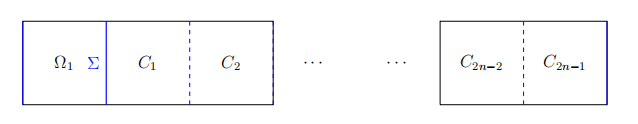
Figure 3: Configuration for case \( n={Z^{+}} \)

\( Tv(x,y)=\begin{cases}\begin{matrix}v(x,y), & if(x,y)∈{Ω_{1}}, \\ -v(x,y)+2v(-x,y), & if(x,y)∈{C_{1}}, \\ -v(x,y)+2v(x-2,y), & if(x,y)∈{C_{2}}, \\ -v(x,y)+2v(-x+2,y), & if(x,y)∈{C_{3}}, \\ -v(x,y)+2v(x-4,y), & if(x,y)∈{C_{4}}, \\ -v(x,y)+2v(-x+4,y), & if(x,y)∈{C_{5}}, \\            ⋮ & \\ -v(x,y)+2v(x-2n+2,y), & if(x,y)∈{C_{2n-2}}, \\ -v(x,y)+2v(-x+2n-2,y), & if(x,y)∈{C_{2n-1}}. \\ \end{matrix}\end{cases} \)

Similarly, we reference the technique used in the case where \( n=2 \) to prove the assumption of the continuous form. Notice that for this generalized case, we ought to prove that each boundary between \( {Ω_{1}} \) and \( {C_{1}} \) , \( {C_{1}} \) and \( {C_{2}} \) , \( {C_{2}} \) and \( {C_{3}} \) , \( … \) , \( {C_{2n-2}} \) and \( {C_{2n-1}} \) are continuous. To generalize and simplify the verification process, we might as well assume for all \( k=1,2,3⋯n \) and prove the continuity that fits every interface within this geometry. We denote that \( {C_{0}} \) is \( {Ω_{1}} \) . Using the same method, we find both limits of each boundary between any \( {C_{2k-2}} \) and \( {C_{2k-1}} \) .

Lemma 3.8. \( Tv \) is continuous on each boundary between any \( {C_{2k-2}} \) and \( {C_{2k-1}} \) .

Proof.

\( \begin{matrix}\underset{\begin{matrix}(x,y)∈{Ω_{1}} \\ x→{(2k-2)^{-}} \\ \end{matrix}}{lim}Tv(x,y) & =\underset{\begin{matrix}(x,y)∈{C_{(2k-2)}} \\ x→{(2k-2)^{-}} \\ \end{matrix}}{lim}(-v(x,y)+2v(x-2k+2,y)) \\ & =-\underset{\begin{matrix}(x,y)∈{C_{(2k-2)}} \\ x→{(2k-2)^{-}} \\ \end{matrix}}{lim}v(x,y)+2\underset{\begin{matrix}(x,y)∈{C_{(2k-2)}} \\ x→{(2k-2)^{-}} \\ \end{matrix}}{lim}v(x-2k+2,y) \\ & =-\underset{\begin{matrix}(x,y)∈{C_{(2k-2)}} \\ x→{(2k-2)^{-}} \\ \end{matrix}}{lim}v(x,y)+2\underset{\begin{matrix}(x,y)∈{Ω_{1}} \\ x→{0^{-}} \\ \end{matrix}}{lim}v(x,y) \\ \end{matrix} \)

\( \begin{matrix}\underset{\begin{matrix}(x,y)∈{C_{(2k-1)}} \\ x→{(2k-2)^{+}} \\ \end{matrix}}{lim}Tv(x,y) & =\underset{\begin{matrix}(x,y)∈{C_{(2k-1)}} \\ x→{(2k-2)^{+}} \\ \end{matrix}}{lim}(-v(x,y)+2v(-x+2k-2,y)) \\ & =-\underset{\begin{matrix}(x,y)∈{C_{(2k-1)}} \\ x→{(2k-2)^{+}} \\ \end{matrix}}{lim}v(x,y)+2\underset{\begin{matrix}(x,y)∈{C_{(2k-1)}} \\ x→{(2k-2)^{+}} \\ \end{matrix}}{lim}v(-x+2k-2,y) \\ & =-\underset{\begin{matrix}(x,y)∈{C_{(2k-1)}} \\ x→{(2k-2)^{+}} \\ \end{matrix}}{lim}v(x,y)+2\underset{\begin{matrix}(x,y)∈{Ω_{1}} \\ x→{0^{-}} \\ \end{matrix}}{lim}v(x,y) \\ \end{matrix} \)

Since \( \underset{\begin{matrix}(x,y)∈{C_{(2k-2)}} \\ x→{(2k-2)^{-}} \\ \end{matrix}}{lim}v(x,y)=\underset{\begin{matrix}(x,y)∈{C_{(2k-1)}} \\ x→{(2k-2)^{+}} \\ \end{matrix}}{lim}v(x,y) \) , therefore, \( \underset{\begin{matrix}(x,y)∈{C_{(2k-2)}} \\ x→{(2k-2)^{-}} \\ \end{matrix}}{lim}Tv(x,y)=\underset{\begin{matrix}(x,y)∈{C_{(2k-1)}} \\ x→{(2k-2)^{+}} \\ \end{matrix}}{lim}Tv(x,y) \) . In conclusion, \( Tv(x,y) \) is continuous on each boundary between any \( {C_{2k-2}} \) and \( {C_{2k-1}} \) .

Lemma 3.9. \( T \) is an isomorphism of \( {V_{per}} \) .

Proof. From Lemma 3.8, we can compute directly

\( \begin{matrix}∥Tv∥_{{V_{per}}}^{2} & =∥∇(Tv)∥_{{L^{2}}({Ω_{1}})}^{2}+∥∇(Tv)∥_{{L^{2}}({Ω_{2}})}^{2} \\ & \\ & =\sum _{i=1}^{2n-1}∥∇(Tv)∥_{{L^{2}}({C_{i}})}^{2} \\ & ≤C∥∇v∥_{{L^{2}}(Ω)}^{2} \\ & =C∥v∥_{{V_{per}}}^{2}. \\ \end{matrix} \)

Therefore, we are able to derive

\( ∥Tv{∥_{{V_{per}}}}≤C∥v{∥_{{V_{per}}}}, \)

which implies that \( Tv(x,y) \) is continuous on \( {V_{per}} \) . To verify the assumption of the bijectivity of \( Tv \) , we again reference the technique of proving \( T(Tv)=Id \) , in this case, \( T(Tv)=v \) . Since

\( Tv(x,y)=\begin{cases}\begin{matrix}v(x,y), & if(x,y)∈{Ω_{1}}, \\ -v(x,y)+2v(-x,y), & if(x,y)∈{C_{1}}, \\ -v(x,y)+2v(x-2,y), & if(x,y)∈{C_{2}}, \\ -v(x,y)+2v(-x+2,y), & if(x,y)∈{C_{3}}, \\ -v(x,y)+2v(x-4,y), & if(x,y)∈{C_{4}}, \\ -v(x,y)+2v(-x,y), & if(x,y)∈{C_{5}}, \\            ⋮ & \\ -v(x,y)+2v(x-2n+2,y), & if(x,y)∈{C_{2n-2}}, \\ -v(x,y)+2v(-x+2n-2,y), & if(x,y)∈{C_{2n-1}}. \\ \end{matrix}\end{cases} \)

Now we calculate each \( T(Tv(x,y)) \) for each region in the geometry, which is displayed in the following process.

\( T(Tv(x,y))=\begin{cases}\begin{matrix}Tv(x,y), & if(x,y)∈{Ω_{1}}, \\ -Tv(x,y)+2Tv(-x,y), & if(x,y)∈{C_{1}}, \\ -Tv(x,y)+2Tv(x-2,y), & if(x,y)∈{C_{2}}, \\ -Tv(x,y)+2Tv(-x+2,y), & if(x,y)∈{C_{3}}, \\ -Tv(x,y)+2Tv(x-4,y), & if(x,y)∈{C_{4}}, \\ -Tv(x,y)+2Tv(-x+4,y), & if(x,y)∈{C_{5}}, \\            ⋮ & \\ -Tv(x,y)+2Tv(x-2n+2,y), & if(x,y)∈{C_{2n-2}}, \\ -Tv(x,y)+2Tv(-x+2n-2,y), & if(x,y)∈{C_{2n-1}}. \\ \end{matrix}\end{cases} \)

To prove the bijectivity of \( T \) , we again assume for all \( k=1,2,3,⋯,n \) and we are going to prove \( T∘T=Id \) . We have:

For all \( (x,y)∈{Ω_{1}} \) ,

\( \begin{matrix}T(Tv(x,y))=v(x,y). \\ \end{matrix} \)

For all \( (x,y)∈{C_{2k-2}} \) ,

\( \begin{matrix}T(Tv(x,y)) & =-Tv(x,y)+2Tv(x-2k+2,y) \\ & =v(x,y)-2v(x-2k+2,y)+2v(x-2k+2,y) \\ & =v(x,y). \\ \end{matrix} \)

For all \( (x,y)∈{C_{2k-1}} \) ,

\( \begin{matrix}T(Tv(x,y)) & =-Tv(x,y)+2Tv(-x+2k-2,y) \\ & =v(x,y)-2v(-x+2k-2,y)+2v(-x+2k-2,y) \\ & =v(x,y). \\ \end{matrix} \)

In brief, it can be concluded as

\( T(Tv(x,y))=\begin{cases}\begin{matrix}v(x,y), & if(x,y)∈{Ω_{1}}, \\ v(x,y), & if(x,y)∈{C_{2k-2}}, \\ v(x,y), & if(x,y)∈{C_{2k-1}}. \\ \end{matrix}\end{cases} \)

Thereby, we show that \( T \) is bijective. Thus, \( T \) is an isomorphism of \( {V_{per}} \) . ◻

Similarly, now we may apply standard techniques to verify that \( a(v,Tv) \) is coercive for some \( κ \) , hence calculating the specific values of \( κ \) where the variational formulation is well-posed. Now we introduce \( {R_{3}}v \) where

\( {R_{3}}v(x,y)=\begin{cases}\begin{matrix}v(-x,y), & if(x,y)∈{C_{1}}, \\ v(x-2,y), & if(x,y)∈{C_{2}}, \\ v(-x+2,y), & if(x,y)∈{C_{3}}, \\    ⋮ & \\ v(x-2n+2,y), & if(x,y)∈{C_{2n-2}}, \\ v(-x+2n-2,y), & if(x,y)∈{C_{2n-1}}. \\ \end{matrix}\end{cases} \)

Therefore,

\( \begin{matrix}a(v,Tv) & ={σ_{1}}\int _{{Ω_{1}}}^{​}{|∇v(x)|^{2}}dxdy+{σ_{2}}\int _{{Ω_{2}}}^{​}∇v(x)\cdot ∇(Tv(x))dxdy \\ & ={σ_{1}}\int _{{Ω_{1}}}^{​}{|∇v(x)|^{2}}dxdy-{σ_{2}}\int _{{Ω_{2}}}^{​}∇{v(x)^{2}}dxdy+2{σ_{2}}\int _{{Ω_{2}}}^{​}(∇v\cdot ∇{R_{3}}v)dxdy \\ & ={σ_{1}}\int _{{Ω_{1}}}^{​}{|∇v(x)|^{2}}dxdy-{σ_{2}}\int _{{Ω_{2}}}^{​}{|∇v(x)|^{2}}dxdy+2{σ_{2}}\int _{{Ω_{2}}}^{​}∇v(x)\cdot ∇({R_{3}}v(x))dxdy. \\ \end{matrix} \)

In this circumstance, we are able to calculate

\( \begin{matrix} & \int _{{Ω_{2}}}^{​}{|∇({R_{3}}v(x))|^{2}}dxdy \\ & =\sum _{j=1}^{n}\int _{{C_{2j-1}}}^{​}{|∇v(-x+2j-2)|^{2}}dxdy+\sum _{j=1}^{n-1}\int _{{C_{2j}}}^{​}{|∇v(x-2j)|^{2}}dxdy \\ & =(2n-1)\int _{{Ω_{1}}}^{​}{|∇v(x,y)|^{2}}dxdy. \\ \end{matrix} \)

Therefore, by applying Young’s Inequality, we have

\( \begin{matrix} & 2|\int _{{Ω_{2}}}^{​}(∇v\cdot ∇({R_{3}}v(x)))dxdy| \\ & ≤2∥∇v{∥_{L_{({Ω_{2}})}^{2}}}\cdot ∥∇{R_{3}}v{∥_{L_{({Ω_{2}})}^{2}}} \\ & ≤2\sqrt[]{2n-1}∥∇v{∥_{L_{({Ω_{1}})}^{2}}}\cdot ∥∇v{∥_{L_{({Ω_{1}})}^{2}}} \\ & ≤\sqrt[]{2n-1}{δ^{-1}}∥∇v∥_{L_{({Ω_{1}})}^{2}}^{2}+\sqrt[]{2n-1}δ∥∇v∥_{L_{({Ω_{1}})}^{2}}^{2} \\ \end{matrix} \)

Then we substitute the inequality above into the original calculation of \( a(v,Tv) \) and we are able to derive

\( \begin{matrix}a(v,Tv)≥({σ_{1}}+\sqrt[]{2n-1}{σ_{2}}δ)\cdot ∥∇v∥_{L_{({Ω_{1}})}^{2}}^{2}-{σ_{2}}(1-\sqrt[]{2n-1}{δ^{-1}})∥∇v∥_{L_{({Ω_{2}})}^{2}}^{2} \\ \end{matrix} \)

Since for \( a(v,Tv) \) , it should always be greater or equal to \( 0 \) . Thereby, we have

\( \begin{matrix}\begin{cases}\begin{matrix}{σ_{1}}+\sqrt[]{2n-1}{σ_{2}}δ \gt 0, \\ 1-\sqrt[]{2n-1}{δ^{-1}} \gt 0. \\ \end{matrix}\end{cases} \\ \end{matrix} \)

After simplifying the calculation, we can deduce the range of \( δ \)

\( \begin{matrix}\begin{cases}\begin{matrix}δ \lt -\frac{{σ_{1}}}{\sqrt[]{2n-1}{σ_{2}}}, \\ δ \gt \sqrt[]{2n-1}. \\ \end{matrix}\end{cases} \\ \end{matrix} \)

We now have the following result: when \( \frac{{σ_{2}}}{{σ_{1}}}∈(\frac{1}{1-2n},0) \) , this variational formulation (3.2) admits a unique solution with reference to Theorem 2.18. This suggests that \( a(v,Tv) \) is coercive in this case, which also implies that it admits a unique solution. However, \( \frac{{σ_{2}}}{{σ_{1}}}∈(\frac{1}{1-2n},0) \) is not the only range for the geometry admitting a unique solution, because \( {σ_{1}} \) and \( {σ_{2}} \) are in equal status and can be reversed. Since this question is an exploration of the asymmetric region, we need to directly construct another \( Tv∈{H^{1}}(Ω) \) , denoted as \( T \prime v \) , to find out the corresponding range for the circumstances to achieve the variational formulation admitting a unique solution. The following process is the construction of \( T \prime v \) , where \( T \prime v:{V_{per}}→{V_{per}} \) , and \( {a_{1}},{a_{2}},{a_{3}},…,{a_{2n-2}},{a_{2n-1}} \) are constants. Then, we construct

\( T \prime v(x,y)=\begin{cases}\begin{matrix}v(x,y)-2w(x,y), & if(x,y)∈{Ω_{1}}, \\ -v(x,y), & if(x,y)∈{Ω_{2}}, \\ \end{matrix}\end{cases} \)

where \( w(x,y)=v(-x,y)+\sum _{i=1}^{n-1}[{a_{2i-1}}v(x+2i,y)+{a_{2i}}v(-x+2i,y)] \) . Similarly, to begin with, we should verify that \( T \prime v \) is continuous on \( Σ \) , so as to obtain the relationship among \( {a_{1}},{a_{2}},{a_{3}},…,{a_{2n-2}},{a_{2n-1}} \) .

\( \begin{matrix}\underset{\begin{matrix}(x,y)∈{Ω_{2}} \\ x→Σ \\ \end{matrix}}{lim}T \prime v(x,y) & =-\underset{\begin{matrix}(x,y)∈{Ω_{2}} \\ x→Σ \\ \end{matrix}}{lim}v(x,y), \\ \underset{\begin{matrix}(x,y)∈{Ω_{1}} \\ x→{0^{-}} \\ \end{matrix}}{lim}T \prime v(x,y) & =\underset{\begin{matrix}(x,y)∈{Ω_{1}} \\ x→{0^{-}} \\ \end{matrix}}{lim}(v(x,y)-2w(x,y)) \\ & =\underset{\begin{matrix}(x,y)∈{Ω_{1}} \\ x→{0^{-}} \\ \end{matrix}}{lim}(v(x,y)-v(-x,y)-\sum _{i=1}^{n-1}[{a_{2i-1}}v(x+2i-2,y)+ \\ & {a_{2i}}v(-x+2i,y)]-{a_{2n-1}}v(-x+2n-2,y)) \\ & =\underset{\begin{matrix}(x,y)∈{Ω_{1}} \\ x→{0^{-}} \\ \end{matrix}}{lim}v(x,y)-2\underset{\begin{matrix}(x,y)∈{C_{1}} \\ x→{0^{+}} \\ \end{matrix}}{lim}v(x,y)-2{a_{1}}\underset{\begin{matrix}(x,y)∈{C_{2}} \\ x→{0^{+}} \\ \end{matrix}}{lim}v(x+2,y)- \\ & 2{a_{2}}\underset{\begin{matrix}(x,y)∈{C_{1}} \\ x→{2^{+}} \\ \end{matrix}}{lim}v(-x+2,y)-⋯2{a_{2n-2}}\underset{\begin{matrix}(x,y)∈{C_{2n-2}} \\ x→{2n-2^{+}} \\ \end{matrix}}{lim}v(x+2n-2,y)- \\ & 2{a_{2n-1}}\underset{\begin{matrix}(x,y)∈{C_{2n-1}} \\ x→{(2n-1)^{+}} \\ \end{matrix}}{lim}v(-x+2n-2,y). \\ \end{matrix} \)

Since the new variational formulation is continuous on \( Σ \) , so \( {lim_{\begin{matrix}(x,y)∈{Ω_{1}} \\ x→{0^{-}} \\ \end{matrix}}}T \prime v(x,y)={lim_{\begin{matrix}(x,y)∈{Ω_{2}} \\ x→{0^{-}} \\ \end{matrix}}}(v(x,y)-2w(x,y)) \) , and we derive the relationship \( {a_{1}}+{a_{2}}+{a_{3}}+⋯+{a_{2n-2}}+{a_{2n-1}}=0 \) . We might as well assume, for any \( k∈N \) , \( {a_{2k+1}}=1 \) and \( {a_{2k}}=-1 \) to simplify our analysis for the well-posedness of this variational formula, where \( T \prime v \) is manifested below:

\( T \prime v(x,y)=\begin{cases}\begin{matrix}v(x,y)-2w(x,y), & if(x,y)∈{Ω_{1}}, \\ -v(x,y), & if(x,y)∈{Ω_{2}}, \\ \end{matrix}\end{cases} \)

where we denote \( w(x,y)=\sum _{j=1}^{n}v(-x+2j-2)+\sum _{j=2}^{n}v(x+2j-2) \) . Now we can show that \( T \prime \) is an isomorphism of \( {V_{per}} \) .

Lemma 3.10. \( T \prime \) is an isomorphism of \( {V_{per}} \) .

Proof. Since \( T \prime v \) is continuous on \( Σ \) , we can directly compute

\( \begin{matrix}∥T \prime v∥_{{V_{per}}}^{2} & =∥∇(T \prime v)∥_{{L^{2}}({Ω_{1}})}^{2}+∥∇(T \prime v)∥_{{L^{2}}({Ω_{2}})}^{2} \\ & =∥∇v(x,y)∥_{{L^{2}}({Ω_{2}})}^{2}+∥∇v(x,y)-2∇w(x,y)∥_{{L^{2}}({Ω_{1}})}^{2} \\ & ≤(2n-1)∥∇v(x,y)∥_{{L^{2}}(Ω)}^{2}. \\ \end{matrix} \)

Therefore, \( ∥T \prime v(x,y){∥_{{V_{per}}}}≤\sqrt[]{2n-1}∥∇v(x,y){∥_{{L^{2}}(Ω)}} \) , which implies that \( T \prime v \) is continuous on \( {H^{1}}(Ω) \) . For the next step, we ought to show that \( T \prime v \) is bijective by proving that \( T \prime (T \prime v)=Id \) , in this case, \( T \prime (T \prime v)=v \prime \) .

\( T \prime v(x,y)=\begin{cases}\begin{matrix}v(x,y)-2w(x,y), & if(x,y)∈{Ω_{1}}, \\ -v(x,y), & if(x,y)∈{Ω_{2}}. \\ \end{matrix}\end{cases} \)

\( T \prime (T \prime v(x,y))=\begin{cases}\begin{matrix}T \prime v(x,y)-2T \prime w(x,y), & if(x,y)∈{Ω_{1}}, \\ -T \prime v(x,y), & if(x,y)∈{Ω_{2}}. \\ \end{matrix}\end{cases} \)

For all \( (x,y)∈{Ω_{1}} \) , we derive

\( \begin{matrix}T \prime v(x,y)-2T \prime w(x,y) & =v(x,y)-2w(x,y)+2w(x,y) \\ & =v(x,y). \\ \end{matrix} \)

For all \( (x,y)∈{Ω_{2}} \) , we have

\( \begin{matrix}-T \prime v(x,y)=v(x,y). \\ \end{matrix} \)

Therefore, \( T \prime \) is bijective. Thus, \( T \prime \) is an isomorphism of \( {V_{per}} \) .

At last, we ought to prove that \( a(v,T \prime v) \) is coercive. Now, we introduce \( {R_{4}}v \) and we define it as \( {R_{4}}v=\sum _{j=1}^{n}v(-x+2j-2)+\sum _{j=2}^{n}v(x+2j-2) \) . Now we have

\( T \prime v(x,y)=\begin{cases}\begin{matrix}v(x,y)-2{R_{4}}v(x,y), & if(x,y)∈{Ω_{1}}, \\ -v(x,y), & if(x,y)∈{Ω_{2}}. \\ \end{matrix}\end{cases} \)

Then we get

\( \begin{matrix}a(u,v) & ={σ_{1}}\int _{{Ω_{1}}}^{​}{|∇{v_{1}}(x)|^{2}}dxdy+{σ_{2}}\int _{{Ω_{2}}}^{​}∇{v_{2}}(x)\cdot ∇(T{v_{2}}(x))dxdy \\ & =-{σ_{2}}\int _{{Ω_{2}}}^{​}{|∇v(x)|^{2}}dxdy+{σ_{1}}\int _{{Ω_{1}}}^{​}∇{v(x)^{2}}-2{σ_{1}}\int _{{Ω_{1}}}^{​}(∇v\cdot ∇{R_{4}}v)dxdy. \\ \end{matrix} \)

In this circumstance, we are able to calculate

\( \begin{matrix} & \int _{{Ω_{2}}}^{​}{|∇({R_{4}}v(x))|^{2}}dxdy \\ & =\sum _{j=1}^{n}\int _{{C_{2j-1}}}^{​}{|∇v(-x+2j-2)|^{2}}dxdy+\sum _{j=1}^{n-1}\int _{{C_{2j}}}^{​}{|∇v(x+2j)|^{2}}dxdy \\ & =(2n-1)\int _{{Ω_{2}}}^{​}{|∇(v(x,y))|^{2}}dxdy. \\ \end{matrix} \)

Therefore, by utilizing Young’s Inequality, we can derive

\( \begin{matrix} & 2|\int _{{Ω_{2}}}^{​}(∇v\cdot ∇(R{v_{1}}(x)))dxdy| \\ & ≤2∥∇v{∥_{L_{({Ω_{2}})}^{2}}}\cdot ∥∇Rv{∥_{L_{({Ω_{2}})}^{2}}} \\ & ≤2\sqrt[]{2n-1}∥∇v{∥_{L_{({Ω_{1}})}^{2}}}\cdot ∥∇v{∥_{L_{({Ω_{1}})}^{2}}} \\ & ≤\sqrt[]{2n-1}{δ^{-1}}∥∇v∥_{L_{({Ω_{1}})}^{2}}^{2}+\sqrt[]{2n-1}δ∥∇v∥_{L_{({Ω_{1}})}^{2}}^{2}. \\ \end{matrix} \)

Then we substitute the inequality above into the original calculation of \( a(v,Tv) \) and we are able to obtain

\( \begin{matrix}a(v,Tv)≥({σ_{1}}-\sqrt[]{2n-1}{σ_{1}}δ)\cdot ∥∇v∥_{L_{({Ω_{1}})}^{2}}^{2}+(-{σ_{2}}-\sqrt[]{2n-1}{σ_{1}}{δ^{-1}})∥∇v∥_{L_{({Ω_{2}})}^{2}}^{2}. \\ \end{matrix} \)

Since for \( a(v,Tv) \) , it should always be greater or equal to \( 0 \) . Thereby, we have

\( \begin{cases}\begin{matrix}-\sqrt[]{2n-1}δ+1 \gt 0, \\ -{σ_{2}}-\sqrt[]{2n-1}{σ_{1}}{δ^{-1}} \gt 0. \\ \end{matrix}\end{cases} \)

With simplification of calculations, we have

\( \begin{matrix}\begin{cases}\begin{matrix}δ \lt \frac{1}{\sqrt[]{2n-1}}, \\ δ \gt -\frac{\sqrt[]{2n-1}{σ_{1}}}{{σ_{2}}}. \\ \end{matrix}\end{cases} \\ \end{matrix} \)

Therefore, for \( T \prime v(x,y) \) , with reference to Theorem 2.18 when \( κ∈(-∞,1-2n) \) , the variational formulation (3.2) has a unique solution. In conclusion, for the general case of variational formulation (3.2) when \( n∈{Z^{+}} \) , it has a unique solution and satisfies the conditions of isomorphism if \( κ∈(-∞,1-2n)∪(\frac{1}{1-2n},0) \) .

References

[1]. X. Shi, A study of non-coercive problems arising from the propagation of elec- tromagnetic waves in metamaterials, 2023 Yau awards 6620.
[2]. F. Albiac, N. Kalton, Topics in Banach Space Theory, Springer, 2006.
[3]. H. Brezis, Functional Analysis, Sobolev spaces and partial differential equa- tions, Springer, universitext ed., 2010.
[4]. Y.Z. Chen, L.C. Wu, Second Order Elliptic Equations and Elliptic Systems, American Mathematical Society, 1998.
[5]. E. DiBenedetto, Partial Differential Equations (2nd ed.), Birkh¨auser, 2009.
[6]. L. C. Evans, Partial Differential Equations, vol. 19 of Graduate Studies in Mathematics, American Mathematical Society, Providence, RI, seconded., 2010.
[7]. P. Lax, Functional Analysis, Wiley, 2002.
[8]. M. Costabel, A coercive bilinear form for Maxwell’s equations, J. Math. Anal. and Appl., 157, 527–541 (1991).
[9]. J.C. N´ed´elec, Acoustic and electromagnetic equations, Applied Mathematical Sciences, 144, Springer, New York (2001).
[10]. V.G. Veselago, The electrodynamics of substances with simultaneously nega- tive values of ε and μ, Soviet Physics-Uspekhi, 10, 509–514 (1968).
Cite this article
Chen,H. (2025). A study of Poisson-type Equations with Sign Changing Parameters in Fully Asymmetric Configurations. Theoretical and Natural Science,87,103-121.
Data availability
The datasets used and/or analyzed during the current study will be available from the authors upon reasonable request.
Disclaimer/Publisher's Note
The statements, opinions and data contained in all publications are solely those of the individual author(s) and contributor(s) and not of EWA Publishing and/or the editor(s). EWA Publishing and/or the editor(s) disclaim responsibility for any injury to people or property resulting from any ideas, methods, instructions or products referred to in the content.
About volume
Volume title: Proceedings of the 4th International Conference on Computing Innovation and Applied Physics
© 2024 by the author(s). Licensee EWA Publishing, Oxford, UK. This article is an open access article distributed under the terms and
conditions of the Creative Commons Attribution (CC BY) license. Authors who
publish this series agree to the following terms:
1. Authors retain copyright and grant the series right of first publication with the work simultaneously licensed under a Creative Commons
Attribution License that allows others to share the work with an acknowledgment of the work's authorship and initial publication in this
series.
2. Authors are able to enter into separate, additional contractual arrangements for the non-exclusive distribution of the series's published
version of the work (e.g., post it to an institutional repository or publish it in a book), with an acknowledgment of its initial
publication in this series.
3. Authors are permitted and encouraged to post their work online (e.g., in institutional repositories or on their website) prior to and
during the submission process, as it can lead to productive exchanges, as well as earlier and greater citation of published work (See
Open access policy for details).