1. Introduction

With the deepening of global concern about climate change, the realization of the "dual carbon" has become a goal pursued by the whole world. To reduce carbon emission, load monitoring has received widespread attention due to its ability to provide detailed power information, which helps users replace inefficient equipment and help grid companies improve the scheduling plan, thus providing safe and accurate services.

Load monitoring is categorized into invasive load monitoring and non-invasive load monitoring (NILM). Invasive load monitoring involves the installation of sensors for each appliance, which is costly. NILM only requires setting up a single sensor to measure the aggregate power consumption of all household appliances. Through disaggregation algorithms, the power consumption of individual appliances is then derived from the total consumption. This concept was firstly introduced by Hart in 1992 [1]. Although its precision may not match the one of invasive methods. its cost-effectiveness and respect for privacy make it more acceptable to the general public, thus attracting considerable attention from researchers.

At present, the commonly used methods for NILM mainly consist of approaches based on the hidden Markov model (HMM) and deep learning methods. Although deep learning methods have high performance in theory, their training process usually requires a lot of time and computational resources. In practical applications, HMM is still a widely adopted choice due to its low computational complexity and ease of implementation. Reference [2] managed to reduce model complexity by introducing the Factorial Hidden Markov Model, and reference [3] further optimized load monitoring performance by integrating Additive FHMM and Differential FHMM. Additionally, reference [4] enhanced the capability to recognize multi-state devices by combining the Multiple Model Probability algorithm with the Additive Differential FHMM.

However, methods above have not fully considered the temporal heterogeneity of the operational states of electrical equipment. This could lead to increased bias in the estimation of HMM parameters, resulting in inaccurate load monitoring when the usage patterns of the devices change. Concerning this issue, we propose a hyper-state HMM modeling method that takes into account the time feature, considering the relationship between the usage time of the devices and the probability distribution of their operational states. This approach allows for a better estimation of HMM parameters, thereby achieving more accurate load monitoring.

2. Problem description and hidden Markov model

2.1. NILM

NILM is the process of monitoring the power consumption of each load from the overall load. Assuming that each load has multiple states and the active power consumption of one load varies significantly between different states, while it is similar within the same state. Therefore, the power consumption of the appliance \( i \) at time \( t \) can be represented as:

\( P_{t}^{i}=\sum _{k=1}^{{K^{i}}}s_{t}^{i,k}{P^{i,k}}\ \ \ (2.1) \)

Where \( {K^{i}} \) is the total number of states that the appliance \( i \) can have, \( s_{t}^{i,k} \) indicates whether the appliance \( i \) is in state \( k \) at time \( t \) , which is a 0-1 variable, and \( {P^{i,k}} \) is the active power associated with state \( k \) of the appliance \( i \) . Assuming the total number of appliances in the house is \( M \) , then the total active power consumed by all appliances at time \( t \) is

\( P_{t}^{all}=\sum _{i=1}^{M}\sum _{k=1}^{{K^{i}}}s_{t}^{i,k}{P^{i,k}}\ \ \ (2.2) \)

Therefore, NILM is equivalent to the process of acquiring \( P_{t}^{i} \) on the basis of \( P_{t}^{all} \) .

2.2. Hyper-state encoding for NILM

In NILM, it is necessary to first classify the state of each load to obtain \( s_{t}^{i,k} \) and \( {P^{i,k}} \) . For this purpose, for each load, the clustering algorithm is used to categorizing its active power into different levels corresponding to different states. To fully utilize the data and limit the complexity of algorithm, we adopt the K-means algorithm. Its basic idea is to divide samples into K clusters by minimizing the distances between samples in the same cluster center. Since the number of clusters K needs to be predetermined, similar power values may be categorized into different states. Therefore, we decrease \( K \) and cluster again once cluster centers are similar. After clustering, the centroids of the clusters equal to \( {P^{i,k}} \) , and K equal to \( {K^{i}} \) .

At any moment, the states of all M loads together form a combination of states. we define this combination as a " hyper-state" and establish a correspondence between the hyper-state and the state combinations by using binary encoding. The specific steps are as follows:

1) Allocate the number of binary encoding digits of each load base on \( {K^{i}} \)

2) Convert each state of every load to a binary representation.

3) Concatenate the binary encodings of each load to obtain the hyper-state encoding.

4) Convert the binary code to decimal, and use it as the encoding for the load's hyper-state.

In this way, by rewriting the hyper-state encoding into binary form and separating it, it is easy to achieve a one-to-one correspondence between the state combination and the hyper-state.

2.3. Problem Modeling

2.3.1. Hidden Markov model. HMM is a statistical model describing stochastic processes with hidden states. In an HMM, the hidden states are not observable, while the observations are visible. The model assumes that observations are independent of each other and that the current state is only related to the previous state.

If we consider hyper-state as hidden state and total electricity meter reading as observation, the course to realize NILM can be transformed into the decoding of an HMM.

2.3.2. HMM in NILM. The method of obtaining parameters for HMM based on hyper-state. Assuming the hyper-state at time t is \( {x_{t}} \) and the total meter reading is \( {O_{t}} \) , the parameters of the HMM can be calculated as follows:

1) State Transition Probability Matrix \( A \) :

\( A[i,j]=P({x_{t}}=j|{x_{t-1}}=i)=\frac{{n_{ij}}}{\sum _{j=1}^{N}{n_{ij}}}\ \ \ (2.3) \)

which indicates the probability of transitioning from hyper-state \( i \) to hyper-state \( j \) between consecutive time points. \( {n_{ij}} \) represents the number of transitions from hyper-state \( i \) to \( j \) , and \( N \) is the total number of hyper-states.

2) Emission Matrix \( B \) :

\( B[j,q]=P({O_{t}}={r_{q}}|{x_{t}}=j)=\frac{{w_{jq}}}{\sum _{q=1}^{Q}{w_{jq}}}\ \ \ (2.4) \)

which shows the probability of the total meter reading being \( {r_{q}} \) when the hyper-states is \( j \) . \( {r_{q}} \) ​ is the \( q-th \) possible reading on the total meter, \( {w_{jq}} \) ​ is the number of occurrences where the hyper-states is \( j \) and the meter reading is \( {r_{q}} \) ​, and \( Q \) is the maximum number of different readings the total meter can have.

3) Initial State Probability Distribution Matrix \( π \) :

\( π[j]=P({x_{t}}=j)=\frac{{v_{j}}}{v}\ \ \ (2.5) \)

which gives the probability of the hyper-state being \( j \) at the initial time. \( {v_{j}} \) is the total count of hyper-states \( j \) , and \( v \) is the sum of occurrences of all hyper-states in the dataset.

3. Time feature based hidden Markov model:

In classical HMMs, model parameters are assumed always same. However, in fact, considering the electricity usage habits of residential households, the parameters vary across different time slots. Therefore, we divide the dataset into different time slots. Load state clustering and HMM parameter calculation is performed separately for each time slot. This approach not only takes into account of the differences in probabilities across different time periods when modeling the HMM, but also limits the possible number of hyper-states that may occur in different time slots, thus reducing the model's spatial complexity.

Viterbi algorithm is a method to find the most probable state sequence in an HMM according to the observed data sequence. The algorithm initializes the path probabilities for each state and then iteratively calculates the maximum probability paths to each state, considering transitions from the previous state and the observation probability of the current state. At the final time point, the algorithm determines the terminating state with the highest probability and reconstructs the entire state sequence by backtracking through previous states.

Traditional Viterbi algorithm assumes precise HMM parameters known, but actually it is impossible to obtain precise parameters. Therefore, we have to consider the probability matrices obtained from historical data as the probability matrices HMM, which leads to accumulated biases over time, as the deviation will continue to accumulate with increasing time. Additionally, the memory required for recording sequences and the time cost for backtracking to find the maximum probability path increase continuously. Moreover, in NILM, it makes little sense to focus on historical appliance states. By contrast, the load state at the current moment is more worthy of attention. Therefore, we simplify the Viterbi algorithm:

1) Simplified Time Series Analysis: Only focus on the current and immediately preceding moments during the NILM process.

2) Elimination of Backtracking: Once the hyper-state for the current moment is determined, avoid backtracking to solve for past states.

Consequently, if the current moment is \( t \) , the specific steps for NILM are as follows:

1) Choose different matrices \( A \) ､ \( B \) ､ \( π \) according to different time slots.

2) Calculate the probability for each hyper-state:

\( {P_{t-1}}[j]=π[j]\cdot B[j,{q_{t-1}}], j=1,2,…,N\ \ \ (3.1) \)

3) Acquire the probabilities for each hyper-state:

\( {P_{t}}[i]=\underset{i}{max}{({P_{t-1}}[j]\cdot A[j,i]\cdot B[i,{q_{t}}])},i=1,2,…,N\ \ \ (3.2) \)

4) Regard \( \underset{i}{{\widetilde{x}_{t}}=argmax}{({P_{t}})} \) as the current hyper-state.

5) Convert the hyper-state to binary format and ascertain the status of each appliance.

6) Estimate the current power for each appliance based on the estimated states.

4. Case study

4.1. Experiment Settings

The AMPds2 dataset [5] is selected to validate the effectiveness of the proposed load NILM method. This dataset is sampled at minute intervals and records the power data of various appliances in a Canadian household over two years, with timestamps annotated.

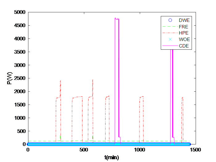
Since the purpose of NILM is to identify the delayed usage of high-power appliances, it is more important to focus on these devices during load monitoring. We conduct experiments using one year of data from five appliances: dishwasher (DWE), refrigerator (FRE), heat pump (HPE), kitchen stove (WOE), and clothes dryer (CDE), selected from the dataset.

In addition to providing power measurement data for each appliance, the AMPds2 dataset also includes the difference between the total household consumption and the measured consumption of each appliance, known as the unknown power loss (UNE). To better reflect real-world scenarios, this paper sets the noise in aggregate load according to it.

4.2. Evaluation Metrics

Accuracy, Multistate F-score, Root Mean Square Error (RMSE) and Estimation Accuracy (Est.Acc) are used to assess the accuracy of load state estimation and load power estimation:

1) Accuracy: represents the proportion of correctly estimated states out of the total states

\( Acc=\frac{Number of correctly estimated samples}{Total number of samples}\ \ \ (4.1) \)

2) F-score for Multiple States:

\( F=2∙\frac{Precision∙Recall}{Precision+Recall}\ \ \ (4.2) \)

\( inacc=\sum _{t=1}^{T}\frac{|\hat{s}_{t}^{i}-s_{t}^{i}|}{{K^{i}}} \)

\( Precision=\frac{tp-inacc}{tp-fp} \)

\( Recall=\frac{tp-inacc}{tp+fn} \)

\( \hat{s}_{t}^{i} \) represents the identified state of the appliance \( i \) at time \( t \) , \( s_{t}^{i} \) is the true state of the appliance \( i \) , where \( tp \) ､ \( fp \) and \( fn \) respectively represent true positive, false positive, and false negative.

3) RMSE: Which represents the differences between predicted values and observed values.

\( RMSE=\sqrt[2]{\frac{1}{T}\sum _{t=1}^{T}{({P_{t}}-{\hat{P}_{t}})^{2}}}\ \ \ (4.3) \)

\( T \) represents the number of samples in the test set, \( {P_{t}} \) is the actual power of the appliance at time \( t \) , and \( {\hat{P}_{t}} \) is the estimated power of the appliance at time \( t \) .

4) Estimation Accuracy

\( Est.Acc=1-\frac{\sum _{t=1}^{T}\sum _{i=1}^{M}|\hat{p}_{t}^{i}-p_{t}^{i}|}{2∙\sum _{t=1}^{M}p_{t}^{i}}\ \ \ (4.4) \)

4.3. Experimental Results

4.3.1. Comparison of Power Estimation Accuracy by Different Methods. This paper employs a 10-fold cross-validation method to evaluate the load monitoring results of the HMM both without considering temporal features and with considering temporal features. The results for each metric are shown in the table below.

Table 1. Load monitoring results without considering time features.

Table 2. Load monitoring results considering time features.

Table 1 and Table 2 respectively present the evaluation results with and without considering the time features. It can be seen that except for FRE, the accuracy of all other appliances is up to 98%. The F-score of DWE in table2 is 30% higher than that in table2. FRE exhibits a more uniform power distribution across the time domain, which makes them less dependent on time features for accurate recognition. By contrast, CDE has a concentrated power consumption pattern in certain time slots. By incorporating time features into the monitoring algorithm, it becomes possible to more effectively identify appliances like CDE.

It can be seen that for WOE, satisfactory results can’t be achieved, regardless of whether temporal features are considered or not. This is primarily due to its low frequency of use and the short duration of each use, which results in low initial probabilities. Additionally, the power used during operation is similar to a specific state of a heat pump (HPE), making it difficult to distinguish its operational state. On the other hand, for other frequently used high-power devices, the load monitoring method described in this paper achieves good accuracy. By considering time features, the calculation criteria for the F-score becomes more stringent due to the more detailed division of states, which may result in a decrease in the F-score for some appliances. However, by this means, the RMSE of each appliance decreases and the Est.Acc increases, which means that this method better establishes the correlation between states and power levels, allowing for more accurate power estimation and reduced error in fact.

4.3.2. Load monitoring Results. The results of load monitoring for all appliances on a certain day in the test set are as follows:

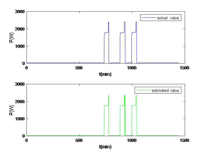
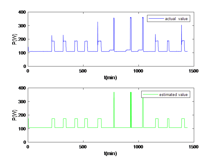
On a certain day, the actual power and the estimated power after monitored for HPE and FRE are as shown in the following diagram:

5. Conclusion

This paper proposes the time feature based hidden Markov model for NILM. Firstly, a hyper-state representation based on binary encoding is defined. Secondly, by considering temporal features, the states of all household appliances within different time periods are modeled as an HMM. To further enhance the efficiency of the algorithm, a simplified Viterbi algorithm is used. On this basis, cross-validation is employed on the AMPds2 dataset to test the HMMs built with and without temporal features under noisy conditions. The case study confirms the advantages of the proposed time-feature based HMM modeling and the simplified Viterbi algorithm, demonstrating their effectiveness in NILM.

References

[1]. Hart G W 1992 Nonintrusive appliance load monitoring Proc. IEEE 80, pp 1870-1891
[2]. Kim H and Marwah M, et al. 2011 Unsupervised Disaggregatio of Low Frequency Power Measurements Proceedings of the 2011 SIAM International Conference on Data Mining. 747-758.
[3]. Kolter Z and Jaakkola T 2012 Approximate Inference in Additive Factorial HMMs with Application to Energy Disaggregation
[4]. Xu Z and Chen W, et al. 2019 A new non-intrusive load monitoring algorithm based on event matching IEEE Access, 7, pp. 55966-55973
[5]. Makonin S and Popowich F 2013 Ampds: A public dataset for load disaggregation and eco-feedback research 2013 IEEE electrical power, IEEE, pp. 1–6.
Cite this article
Sun,Y. (2025). Time feature based hidden Markov model for NILM. Theoretical and Natural Science,95,80-86.
Data availability
The datasets used and/or analyzed during the current study will be available from the authors upon reasonable request.
Disclaimer/Publisher's Note
The statements, opinions and data contained in all publications are solely those of the individual author(s) and contributor(s) and not of EWA Publishing and/or the editor(s). EWA Publishing and/or the editor(s) disclaim responsibility for any injury to people or property resulting from any ideas, methods, instructions or products referred to in the content.
About volume
Volume title: Proceedings of the 2nd International Conference on Applied Physics and Mathematical Modeling
© 2024 by the author(s). Licensee EWA Publishing, Oxford, UK. This article is an open access article distributed under the terms and
conditions of the Creative Commons Attribution (CC BY) license. Authors who
publish this series agree to the following terms:
1. Authors retain copyright and grant the series right of first publication with the work simultaneously licensed under a Creative Commons
Attribution License that allows others to share the work with an acknowledgment of the work's authorship and initial publication in this
series.
2. Authors are able to enter into separate, additional contractual arrangements for the non-exclusive distribution of the series's published
version of the work (e.g., post it to an institutional repository or publish it in a book), with an acknowledgment of its initial
publication in this series.
3. Authors are permitted and encouraged to post their work online (e.g., in institutional repositories or on their website) prior to and
during the submission process, as it can lead to productive exchanges, as well as earlier and greater citation of published work (See
Open access policy for details).