


1. Introduction
1.1. Background and Significance
In 1959, humans successfully created the world's first industrial robot "Unimate". Since then, more and more people have paid attention to the field of robotics, which has flourished and demonstrated its application scenarios and development potential. This type of robot is the culmination of many elements such as mechanics, electronics, materials, control, software, and is also a typical representative of the combination of automation and traditional machinery [1]. The emergence of robots not only greatly liberates productivity and reduces the need for people to engage in monotonous, heavy, and dangerous work, but also improves labor productivity and product quality.
Experts in the field of robotics in our country classify robots into two categories from the perspective of their application environment: industrial robots and specialized robots [2]. At present, robots are mainly used in the following fields: industrial automation production, agriculture, forestry, animal husbandry, sideline and fishery, military applications, special operations, harsh working environments and hazardous work areas.
Due to the vast development market of industrial robots and their ability to greatly improve efficiency and quality in production work, this article conducts kinematic and dynamic simulation analysis on common four axis robotic arms, making them versatile in design and control function implementation.
2. Kinematic analysis of a four axis robotic arm
2.1. Overview of kinematics of four axis robotic arm
This four axis robotic arm is a series connected robotic arm, which is a spatial open chain linkage mechanism composed of a series of linkages and has four degrees of freedom. In a four axis robotic arm, it has a fixed end and a free end, where the fixed end is fixedly connected to the base and the free end is equipped with an end effector, which can be used to perform a certain practical operation. The remaining linkages are connected by different motion pairs to form different joints, and multiple linkages are combined to drive the end effector to move to the specified pose (position and posture). The relationship between the variables of each joint in the kinematic study of a four axis robotic arm and the attitude and position of the end effector in space can provide theoretical basis and research methods for trajectory planning of the robotic arm in the later stage [4].
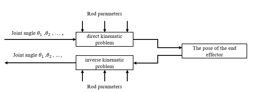
The research problems of four axis robotic arms mainly include two types: forward kinematics problems and inverse kinematics problems [5].
• Kinematic forward problem: Given a given robotic arm, if the geometric parameters of the arm and the vector of its joint angles are known, the pose of the end effector relative to the reference coordinate system (usually a fixed coordinate system) can be obtained.
• Inverse kinematics problem: Given a given robotic arm, if the geometric parameters of the robotic arm and the expected pose of the end effector relative to the reference coordinate system are known, the joint angle vector of the robotic arm moving to the specified pose can be obtained.
|
|
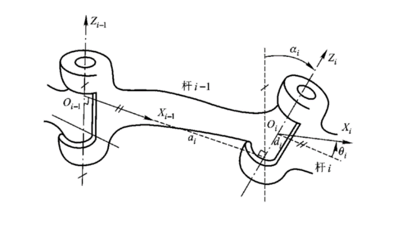
Figure 1. Figure with the relationship between forward and inverse kinematics problems. | Figure 2. Figure with establishment of coordinate system for robot arm connecting rod. |
2.2. Forward kinematics analysis of a four axis robotic arm
2.2.1. D-H method represents kinematic equations
The kinematics of a robotic arm mainly studies the relationship between variables in each joint and the position and attitude of its end effector. By establishing coordinate systems in each joint, the position and orientation of the end effector relative to the reference coordinate system are derived from the interrelationships in these coordinate systems. This article uses the four parameter method, namely the D-H method, to derive the kinematic equations.
Establish the coordinate system of each joint as shown in Figure 2 using the D-H parameter method [6]. Set the coordinate system \( \lbrace i-1\rbrace \) of rod \( i-1 \) on joint \( i-1 \) and fix it to rod \( i-1 \) . Similarly, the coordinate system \( \lbrace i\rbrace \) of rod \( i \) is set on joint \( i \) and is fixedly connected to rod \( i \) [4].
According to the principle of coordinate transformation and combined with Figure 2 analysis, it can be concluded that the coordinate system \( \lbrace i-1\rbrace \) is translated along the \( {x_{i-1}} \) axis by a distance of \( {a_{i-1}} \) , rotated around the \( {x_{i-1}} \) axis by \( {a_{i-1}} \) degrees, and translated along the \( {z_{i}} \) axis by a distance of \( {d_{i}} \) and finally rotated around the \( {z_{i}} \) axis by \( {θ_{i}} \) degrees. Thus, the coordinate system \( \lbrace i\rbrace \) has been obtained. The four D-H parameters involved in the transformation are defined in Table 1.
Table 1. D-H parameter definition table.
Parameter | meaning |
\( {a_{i-1}} \) | The distance between the Z-axis of two joints along their common normal, with the \( {x_{i-1}} \) axis as the positive direction |
\( {α_{i-1}} \) | The angle between two axes in a plane perpendicular to the length of the rod, with counterclockwise rotation of the \( {x_{i-1}} \) axis as the positive direction |
\( {d_{i}} \) | The distance between two adjacent connecting rods along the Z-axis direction, with the \( {z_{i}} \) axis as the positive direction |
\( {θ_{i}} \) | The angle between two adjacent connecting rods in the Z-axis direction, with counterclockwise rotation of the \( {z_{i}} \) axis as the positive direction |
Write the matrix during the transformation from coordinate system \( \lbrace i-1\rbrace \) to coordinate system \( \lbrace i\rbrace \) using the method of single step homogeneous transformation matrix:
(1) Translate the distance of segment \( {a_{i-1}} \) along the \( {x_{i-1}} \) axis:
;
(2) Rotate \( {α_{i-1}} \) degrees around the \( {x_{i-1}} \) axis:
;
(3) Translate the \( {d_{i}} \) segment distance along the \( {z_{i}} \) axis:
;
(4) Rotate \( {θ_{i}} \) degrees around the \( {z_{i}} \) axis:
Finally, through the above four transformations, the pose matrix of adjacent rods can be obtained as follows:
2.2.2. Establishment of forward kinematics equations for a four axis robotic arm
The research object of this article is a four axis robotic arm, which is modeled in 3D in Solidworks, as shown in Figure 3. A robotic arm consists of four parts, namely the waist (lumbar joint), upper arm (shoulder joint), lower arm (elbow joint), and wrist (wrist joint). At the same time, the rotation of each joint is driven by the joint motor DM-J8009-2EC of Damao. The core chip in the control development board is STM32F407IGH6TR.
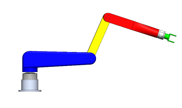
Figure 3. Figure with three dimensional model of four axis robotic arm
Based on the method of establishing a coordinate system in 2.2.1, establish the physical 3D model in Figure 3 as the coordinate system shown in Figure 4, and take the coordinate system of the first joint to coincide with the base coordinate system. According to the D-H parameter representation in 2.2.1, the linkage parameters and joint variables in Table 2 can be obtained.
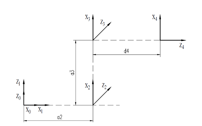
Figure 4. Figure with simplified coordinate system diagram
Table 2. Link parameters and joint variables of a four axis robotic arm.
\( i \) | \( {θ_{i}} \) /(°) | \( {α_{i-1}} \) /(°) | \( {d_{i}} \) /(mm) | \( {a_{i-1}} \) /(mm) | Range of \( {θ_{i}} \) /(°) |
1 | \( {θ_{1}} \) | 0 | 0 | 0 | -150~150 |
2 | \( {θ_{2}} \) | -90 | 0 | \( {a_{2}} \) (400) | -135~0 |
3 | \( {θ_{3}} \) | 0 | 0 | \( {a_{3}} \) (300) | -45~45 |
4 | \( {θ_{4}} \) | -90 | \( {d_{4}}(-350) \) | 0 | -135~135 |
Substitute the parameters in Table 2.2 into the linkage change matrix obtained in 2.2.1, and use Matlab to calculate the matrix to obtain the transformation matrices of the four linkages:
The pose in the coordinate system related to the end effector of a four axis robotic arm can be obtained by \( {_4^0}T={_1^0}T{_2^1}T{_3^2}T{_4^3}T \) :
Among them, \( {c_{i}}=cos{θ_{i}} \) , \( {c_{ij}}=cos{(θ_{i}}+{θ_{j}}) \) , \( s=sin{θ_{i}} \) , \( {s_{ij}}=sin{(θ_{i}}+{θ_{j}}) \) , and \( \vec{n} \) is the normal vector of the end effector, o ⃗ is the orientation vector of the end effector, and a ⃗ is the approach vector of the end effector. These three vectors form the right-hand rule, that is, \( \vec{n}=\vec{o}×\vec{a} \) , and finally, \( {p_{x}} \) , \( {p_{y}} \) and \( {p_{z}} \) are the coordinates of the end effector in the reference coordinate system [4].
Equation (2-2) is the positive solution for the four axis robotic arm. If the initial position data is taken, \( {a_{2}}=400mm, {a_{3}}=300mm, {d_{4}}=-350mm,{ θ_{1}}={θ_{3}}={θ_{4}}=0°,{ θ_{2}}=-90° \) .Substituting (2-2) yields the initial pose as:
This is consistent with the coordinates of the initial pose of the four axis robotic arm shown in Figure 3, successfully verifying the accuracy of equation (2-2).
2.3. Inverse kinematics analysis of four axis robotic arm
In this article, the inverse transformation method is used, which is a type of algebraic method. Its advantage is that it can obtain all solutions without the need for initial values [7]. The basic idea is to sequentially multiply the inverse matrix of the pose matrix obtained in 2.2 by the motion equation of the robot, in order to obtain the values of the variables of each joint.
Firstly, calculate the inverse matrix of each linkage transformation matrix:
(1) Solve \( {θ_{1}} \) :
Using the left multiplication equation (2-2), we obtain:
\( {_1^0}{T^{-1}}{_4^0}T={_4^1}T \)
You can obtain:
Expanding equation (2-3) includes:
By making the (2,4) on both sides of the equation equal, we can obtain:
From equation (2-5), we can obtain:
(2) Solve \( {θ_{2}} \) :
Substitute (1,3) in equation (2-2) into (1,4) in equation (2-2), while making both sides of the equation equal:
Then,
Further calculations reveal that:
According to the angle range in Table 2, it can be seen that \( {θ_{2}} \) can only be negative. Therefore:
(3) Solve \( {θ_{3}} \) :
By making the equation of (3,3) in equation (2-2) equal on both sides, we can obtain:
Then,
Substituting equation (2-10) into equation (2-12) yields:
(4) Solve \( {θ_{4}} \) :
By making the equations (3,1) and (3,2) in equation (2-2) equal on both sides and combining them, we can obtain:
Then,
Finally calculated:
Thus, the inverse kinematics solution of the four axis robotic arm has been obtained, expressed as equations (2-6), (2-10), (2-13), and (2-16).
2.4. Matlab kinematic simulation of four axis robotic arm
In section 2.1, the coordinates of the end effector pose of the robotic arm were obtained by substituting special values, and the results of the kinematic forward solution were verified. However, this method is not universal and not intuitive. Therefore, the motion simulation of the four axis robotic arm is now analyzed.
This simulation analysis uses the Robotics Toolbox toolbox in Matlab, which integrates a large number of robot development and research functions, enabling simulation of robot kinematics, dynamics, trajectory generation, and path planning [8].
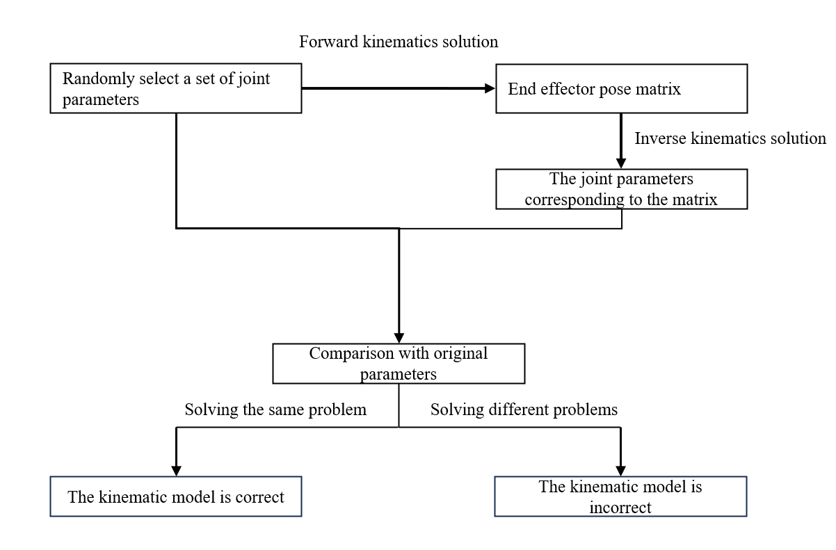
Use the functions in the Robotics Toolbox toolbox to solve the forward and inverse kinematics of the robotic arm, and compare the results with the motion equation solutions in sections 2.2 and 2.3 to verify the correctness of the model. As shown in Figure 5, the verification flowchart for solving forward and reverse motion is presented.
|
|
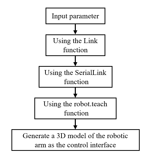
Figure 5. Figure with flowchart for verifying the solution of forward and reverse motion | Figure 6. Figure with Matlab kinematic simulation step slow chart |
2.4.1. Establishment of simulation model
Perform kinematic simulation on the four axis robotic arm, as shown in Figure 6 which is the simulation process flowchart.
Create the object model of the four axis robotic arm in Matlab, as shown in Figure 7, which shows the initial pose of the four axis robotic arm.
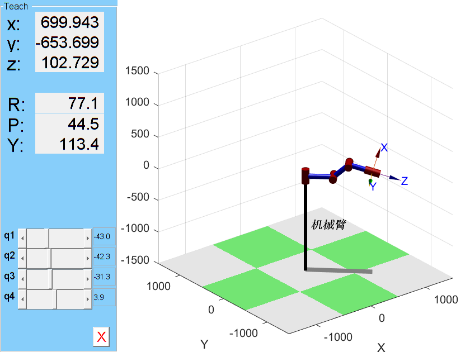
Figure 7. Figure with Matlab simulation model
2.4.2. Verification of forward and inverse kinematics solutions
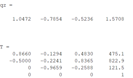
The fkin function in the Robotics Toolbox can be called to solve the forward solution of the motion of a robotic arm. Take the joint vector of the starting point of the four axis robotic arm as qz = [pi/3 pi/4 pi/6 pi/2], substitute it into the calculation, and the Matlab calculation result is shown in Figure 8. At the same time, substituting the joint vectors into equation (2-2) and computing in Matlab yields the solution shown in Figure 9 [9].
|
|
Figure 8. Figure with fkine function calculation result | Figure 9. Figure with calculation results of positive motion equation |
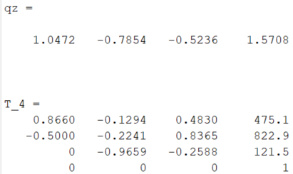
After comparison, it was found that the same calculation results can prove the correctness of the forward motion equation.
The ikine function in the Robotics Toolbox can be called to solve the inverse solution of the motion of a robotic arm. Since the degree of freedom of the four axis robotic arm is 4, M can be set to [1 1 1 0]. If the joint vector of the initial position of the robotic arm is q = [0 pi/200 0], and the homogeneous transformation matrix of the joint coordinates endpoint of the end effector is known as:
Substitute the Matlab operation results into the ikine function as shown in Figure 10. At the same time, the homogeneous transformation matrix of the joint coordinate endpoints of the end effector is substituted into equations (2-6), (2-10), (2-13), and (2-16), and the solution obtained by computing in Matlab is shown in Figure 11 [9].
|
|
Figure 10. Figure with ikine function calculation result | Figure 11. Figure with results of inverse kinematics calculation |
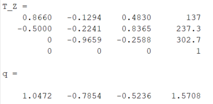
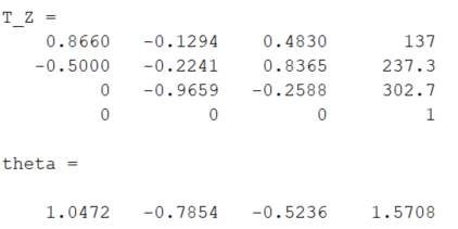
After comparison, it was found that the same calculation results can prove the correctness of the inverse motion equation.
2.5. Analysis of the workspace of a four axis robotic arm
This article uses Monte Carlo method to simulate the workspace of the four axis robotic arm, which can intuitively represent the workspace of the robotic arm. The steps of this method are shown in Figure 12.
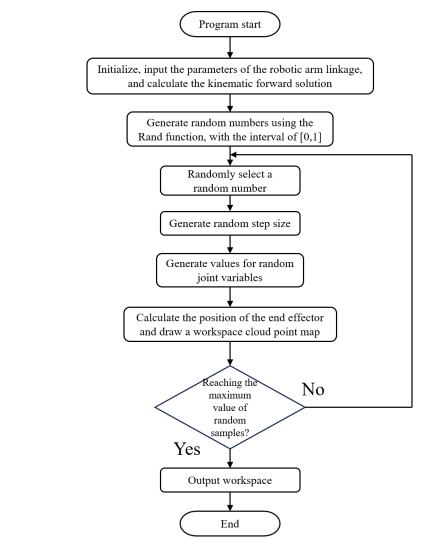
Figure 12. Figure with flowchart of the simulation program for the workspace of a robotic arm
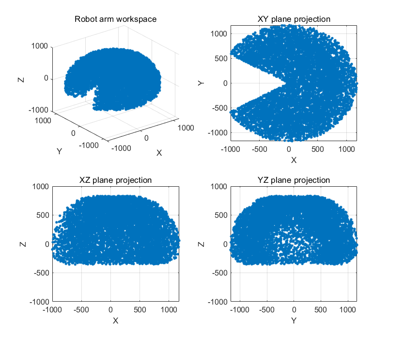
According to equation (2-2) and the rotation range of each joint in Table 2, use Monte Carlo method to simulate the programming workspace in Matlab, with a sample size of 10000. Finally, the point cloud map of the workspace and the projection maps of three coordinate planes were obtained as shown in Figure 13.
It is easy to observe from Figure 13 that under this angle constraint, the workspace of the four axis robotic arm can be approximated as a semi ellipsoid. Due to the limitation of the working range under this condition, there is a fan-shaped gap on one side of the semi ellipsoid. The range of the workspace can be directly read from Figure 13 to determine whether the geometric dimensions of the four axis robotic arm meet the work requirements.
However, due to the limitations of actual size, there are still positions inside the semi ellipsoidal space that cannot be reached by the robotic arm. In order to more intuitively display these unreachable positions, this article uses Matlab to draw the xoy section diagram as shown in Figure 14.
|
|
Figure 13. Figure with point cloud map of workspace and projection of three coordinate planes | Figure 14. Figure with xoy sectional view of workspace |
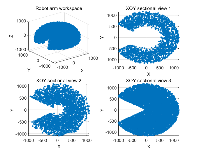
It is easy to observe from Figure 14 that there is a cavity in the workspace near the Z-axis center, and there are no obvious cavities or voids at the center of each axis, which is in line with the angle range set for each joint of the four axis robotic arm.
3. Dynamic analysis of a four axis robotic arm
3.1. Lagrangian Dynamics Analysis
This article uses the Lagrangian dynamics method [10] to analyze a four axis robotic arm. The Lagrangian function \( L \) can be expressed as the difference between the system's kinetic energy \( {E_{k}} \) and potential energy \( {E_{p}} \) . Based on the Lagrangian function \( L \) , the Lagrangian equation of the system can be written as follows:
Firstly, in addition to the kinetic energy of the rods, considering the presence of driving and transmission components in the robot system, the total kinetic energy of the calculated mechanism is:
In the formula, \( H(q) \) represents the inertia matrix of the robot, and in its elements \( {h_{jk}}=\sum _{i=max\lbrace j,k\rbrace }^{n}Trace[\frac{∂{T_{i}}}{∂{q_{j}}}{J_{i}}\frac{∂{{T_{i}}^{T}}}{∂{q_{j}}}] \) , \( q \) and \( {q_{i}} \) represent the joint angles and angular velocities of the four axis robotic arm, where \( n \) is a vector; \( {I_{a}} \) represents the equivalent transmission inertia vector of the robotic arm joint transmission device.
Secondly, the total potential energy of the calculation institution is:
In equation (3-3), \( {m_{i}} \) is the mass of member \( {L_{i}} \) ; \( {r_{i}} \) is the radial axis of member \( {L_{i}} \) in its rigid body coordinate system; represents the gravitational acceleration vector, i.e. .
Finally, equations (3-2) and (3-3) were substituted into equation (3-1) to obtain the final Lagrangian kinematic equation
In the formula,
Subsequently, the Lagrangian equation was used to model the dynamics of the four axis robotic arm. As the fourth degree of freedom of the robotic arm is the rotation of the end effector, it has no impact on the overall dynamics modeling. The solid three-dimensional model was abstracted into a theoretical model as shown in Figure 15.
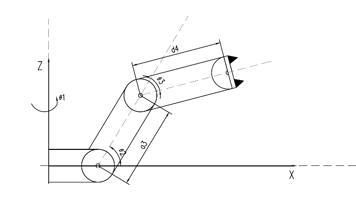
Figure 15. Figure with simplified model of four axis robotic arm
According to equation (3-2), the total kinetic energy of the system is obtained as
According to equation (3-3), the potential energy of the system is obtained as
The Lagrange function obtained from equations (3-8) and (3-9) is
Solving the dynamic equations of four generalized coordinates separately and represent them in matrix form,
Among them,
Equation (3-11) is the dynamic equation of the four axis robotic arm.
3.2. Admas dynamic simulation analysis
In order to have a clearer and more intuitive understanding of the dynamic performance of the four axis robotic arm, this article uses Admas to simulate the dynamics of the model established. The process of this dynamic simulation is shown in Figure 16 [11].
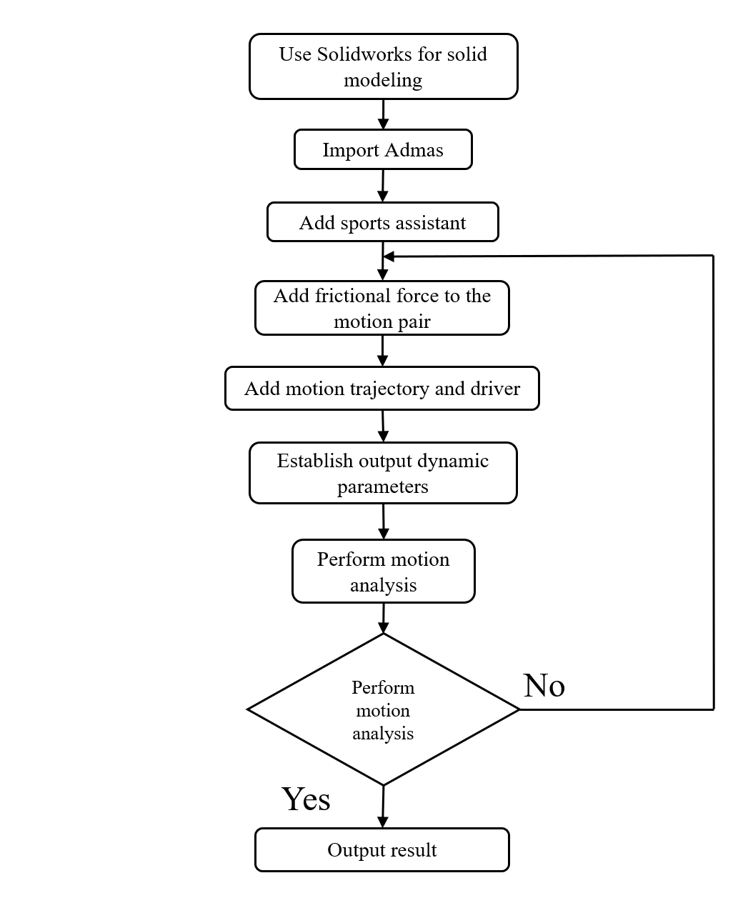
Figure 15. Figure with Admas dynamic simulation flowchart
Import the solid model from Solidworks into Admas and add motion pairs and forces on various components, such as gravity, friction, etc. Obtain the simulation model shown in Figure 16 in Admas.
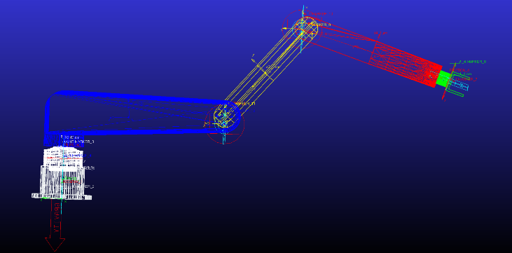
Figure 16. Figure with Admas simulation model
By setting various motion parameters and adding motion trajectories and drivers, the torque, angular velocity, and angular acceleration curves of each joint corresponding to the end effector of the four axis robotic arm moving at a speed of 50m/s along a straight line from points (-67.56, -794, -405) to (732.78, -718, -385) are shown in Figure 17.
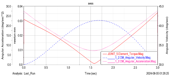
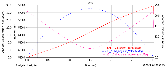
(a) Lumbar joint (b) Arm joint
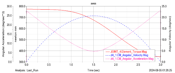
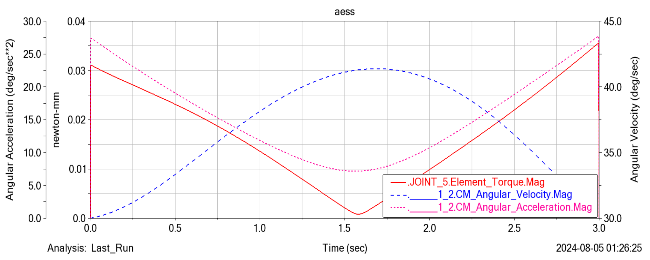
(c) Forearm joint (d) Wrist joint
Figure 16. Figure with curve graph of torque, angular velocity, and angular acceleration of each joint
By observing the image, it is not difficult to find that as the number of elements in the lumbar joint decreases over time, the velocities of other joints increase as the angular velocity of the lumbar joint decreases; For the same joint, the higher the movement speed, the greater its angular velocity; The smaller the speed, the greater the required driving force; The slope change of angular velocity represents the change of angular acceleration.
4. Summarize
With the quiet arrival of Industry 4.0, the demand for robotic arms, which have high production efficiency and product qualification rate, is increasing day by day. More small and medium-sized enterprises in China are introducing robot technology. In order to lower the technological threshold and improve production efficiency. This article introduces a general method for studying the kinematic and dynamic problems of a four axis robotic arm:
(1) By establishing a D-H kinematic model, the general solution for the forward and inverse kinematics of a general four axis robotic arm was obtained, and its kinematic equations were derived using matrix transformation. Simultaneously use the Robotics Toolbox in Matlab to verify the obtained kinematic forward and inverse solutions.
(2) By using the obtained forward and inverse kinematics solutions, a point cloud map of the workspace of the four axis robotic arm was drawn using Monte Carlo method, providing a clearer observation of the workspace range of the four axis robotic arm.
(3) The Lagrangian dynamics method was used to establish the dynamic equations of a four axis robotic arm. The 3D solid model from Solidworks was imported into Admas for dynamic analysis, and images of the torque, angular velocity, and angular acceleration experienced by each joint during specified motion were plotted.
This article mainly focuses on the theoretical stage of research on four axis robotic arms, providing a foundation for further in-depth research.
References
[1]. Zhao Jiangtian. Research on the Application and Development of Industrial Robot Technology in Intelligent Manufacturing [J]. Automation Applications, 2023(7): 16-18.
[2]. Dai Haocen, Sun Danning and Zhao Wenbo. A Review of the Development and Application of Industrial Robot Technology [J]. New Industrialization, 2021, 11(04): 5-6.
[3]. Liu Yicai and Gao Jun. Research on the Current Situation and Countermeasures of Industrial Robot Industry Development [J]. China Business Theory, 2021(18): 174-176.
[4]. Zhou Fei Research on Motion Simulation of Four Degree of Freedom Joint Robot Arm [Master's Thesis] Nanjing: Nanjing University of Aeronautics and Astronautics, 2015.
[5]. Xie Jia, Dou Lianghao, Li Yongguo, et al. Motion analysis and trajectory planning of a five degree of freedom robotic arm [J]. Manufacturing Automation, 2022.44 (7): 11-15.
[6]. Xiong Youlun, Li Wenlong and Chen Wenbin. Robotics Modeling, Control, and Vision [M]. Wuhan: Huazhong University of Science and Technology Press, 2018.
[7]. JIN M, LIU Q, WANG B, et al. An efficient and accurate inverse kinematics for 7-DOF redundant manipu-lators based on a hybrid of analytical and numerical method [J]. IEEE Access, 2020, 8(5):16316- 16330.
[8]. Wang Dachao, Liu Hong. Simulation analysis of robotic arm based on MATLAB and ADAMS [J]. Mechanical Engineering and Automation, 2017 (6): 59-60, 62
[9]. Zhou Rui, Li Shuying, Wang Yibo, et al. Kinematic Analysis of a 5-DOF Manipulator [J]. Tool Technology, 2020, 54(8): 45-49.
[10]. Xia Wei, Zhang Yan. Six degree of freedom machine based on SolidWorks and ADMAS Research on Joint Simulation of Robotic Arms [J]. Mechanical Engineering and Automation, 2021, 45 (5):79-81.
[11]. Shi Chen and Lei Lei. Research on Dynamic Simulation of Picking Robot Based on ADAMS Research on Agricultural Mechanization, 2021, 43 (8): 31-35.
Cite this article
Liao,C. (2025). Kinematic and dynamic analysis of a four axis robotic arm. Theoretical and Natural Science,95,110-124.
Data availability
The datasets used and/or analyzed during the current study will be available from the authors upon reasonable request.
Disclaimer/Publisher's Note
The statements, opinions and data contained in all publications are solely those of the individual author(s) and contributor(s) and not of EWA Publishing and/or the editor(s). EWA Publishing and/or the editor(s) disclaim responsibility for any injury to people or property resulting from any ideas, methods, instructions or products referred to in the content.
About volume
Volume title: Proceedings of the 2nd International Conference on Applied Physics and Mathematical Modeling
© 2024 by the author(s). Licensee EWA Publishing, Oxford, UK. This article is an open access article distributed under the terms and
conditions of the Creative Commons Attribution (CC BY) license. Authors who
publish this series agree to the following terms:
1. Authors retain copyright and grant the series right of first publication with the work simultaneously licensed under a Creative Commons
Attribution License that allows others to share the work with an acknowledgment of the work's authorship and initial publication in this
series.
2. Authors are able to enter into separate, additional contractual arrangements for the non-exclusive distribution of the series's published
version of the work (e.g., post it to an institutional repository or publish it in a book), with an acknowledgment of its initial
publication in this series.
3. Authors are permitted and encouraged to post their work online (e.g., in institutional repositories or on their website) prior to and
during the submission process, as it can lead to productive exchanges, as well as earlier and greater citation of published work (See
Open access policy for details).
References
[1]. Zhao Jiangtian. Research on the Application and Development of Industrial Robot Technology in Intelligent Manufacturing [J]. Automation Applications, 2023(7): 16-18.
[2]. Dai Haocen, Sun Danning and Zhao Wenbo. A Review of the Development and Application of Industrial Robot Technology [J]. New Industrialization, 2021, 11(04): 5-6.
[3]. Liu Yicai and Gao Jun. Research on the Current Situation and Countermeasures of Industrial Robot Industry Development [J]. China Business Theory, 2021(18): 174-176.
[4]. Zhou Fei Research on Motion Simulation of Four Degree of Freedom Joint Robot Arm [Master's Thesis] Nanjing: Nanjing University of Aeronautics and Astronautics, 2015.
[5]. Xie Jia, Dou Lianghao, Li Yongguo, et al. Motion analysis and trajectory planning of a five degree of freedom robotic arm [J]. Manufacturing Automation, 2022.44 (7): 11-15.
[6]. Xiong Youlun, Li Wenlong and Chen Wenbin. Robotics Modeling, Control, and Vision [M]. Wuhan: Huazhong University of Science and Technology Press, 2018.
[7]. JIN M, LIU Q, WANG B, et al. An efficient and accurate inverse kinematics for 7-DOF redundant manipu-lators based on a hybrid of analytical and numerical method [J]. IEEE Access, 2020, 8(5):16316- 16330.
[8]. Wang Dachao, Liu Hong. Simulation analysis of robotic arm based on MATLAB and ADAMS [J]. Mechanical Engineering and Automation, 2017 (6): 59-60, 62
[9]. Zhou Rui, Li Shuying, Wang Yibo, et al. Kinematic Analysis of a 5-DOF Manipulator [J]. Tool Technology, 2020, 54(8): 45-49.
[10]. Xia Wei, Zhang Yan. Six degree of freedom machine based on SolidWorks and ADMAS Research on Joint Simulation of Robotic Arms [J]. Mechanical Engineering and Automation, 2021, 45 (5):79-81.
[11]. Shi Chen and Lei Lei. Research on Dynamic Simulation of Picking Robot Based on ADAMS Research on Agricultural Mechanization, 2021, 43 (8): 31-35.