1. Introduction

The Markov chain, first proposed by the Russian mathematician Markov in 1906, was initially used for the study of linguistic statistics. Markov described the probability of the occurrence of words by using a sequence of random variables. Subsequently, Kolmogorov laid the theoretical foundation for it. Later, Metropolis proposed Markov Chain Monte Carlo, and Baum and other researchers proposed hidden Markov Model. Concepts such as the Markov decision process appeared successively. The current hot issues of Markov process concentrate on firstly, the integration of Markov chains with cutting-edge technologies such as deep learning to extract more value from data. Secondly, in high-dimensional and complex data scenarios, the further optimization of Markov chain algorithms to improve computational efficiency and model generalization ability. Thirdly, the expansive applications of Markov chains in emerging fields, such as quantum computing and brain science, providing new methods and ideas for interdisciplinary research.

Previous studies and literatures have shown that Markov chain can be used extensively in the field of computer science. For instance, Qian et al. use improved Markov chain to construct efficient domain name generation algorithm [1]. Chelly et al. utilize the Markov chain-based generation flow network to achieve consistent amortized clustering [2]. Li et al. have researched the combination of deep computer technique and Markov theorem for deep computerized adaptive testing to revolutionize contemporary assessment practices in education and behavioral health by dynamically adapting test material to meet individual examinees' needs during the evaluation process [3]. Further, Chen et al. have researched for using Markov chain to select important nodes in random network by creating efficient sampling procedure [4]. The importance of exploring the applications of Markov chain lies in improving data manipulation in digital age.

This paper is structured as follows. Section 2 will introduce some basic method and theory with the inclusion of the definition of Markov process and some properties of Markov chain. Section 3 will present some background information about the importance of using Markov chains and introduce two famous applications of Markov chain in the transformation of cloud service trusted state and the prediction of network traffic. Section 4 will conclude the paper with summaries of the findings and the expectations for future researches.

2. Method and Theory

2.1. Definition of Markov Process

Markov process is a probabilistic process that is used to model systems where the state that will occur in the future is contingent solely upon the present state and has no connection or reliance on the state that preceded it. Given the present state in order to predict the future state.

The two main types of Markov process are discrete Markov process and continuous Markov process. For a discrete Markov process, the parameter takes discrete values which are usually represented by the set of integers ( \( n=0,1,2,⋯, \) ) and the state space is usually discrete. It is clear that discrete time points are used to observe the change of system's state. It is suitable for the analysis of web browsing behavior and text generation. For a continuous Markov process, the time parameter takes continuous values which are usually represented by the set of non-negative real numbers ( \( t≥0 \) ), and the state space is usually continuous. It means that the system state can be observed at any moment. It is often used in field such as queuing theory and the dynamics of biological populations.

In this paper, the author mainly focused on analyzing the Discrete Markov process. The mathematical definition of Discrete Markov process is that concerning a succession of random variables \( {X_{1}},{X_{2}},⋯,{X_{n}} \) , for all \( n ≥ 0 \) , and for all possible values \( {x_{1}},{x_{2}},⋯,{x_{n}} \) of the random variables, satisfy the following formula

\( P({X_{n+1}}={x_{n+1}}|{X_{n}}={x_{n}},{X_{n-1}}={x_{{n_{1}}}},⋯,{X_{0}}={x_{0}})=P({X_{n+1}}|{x_{n+1}})\ \ \ (1) \)

A Markov process is often typified by a transition probability matrix \( P \) . Each element, which denoted by \( {P_{ij}} \) , in the matrix \( P \) denotes the probability by which there is a shift from state \( i \) to state \( j \) in one state. It satisfies the following relation

\( {P_{ij}}=P({X_{n+1}}={x_{j}}|{X_{n}}={x_{i}})\ \ \ (2) \)

The form of the transition probability matrix is thus \( P=(\begin{matrix}{P_{00}} & ⋯ & {P_{0n}} \\ ⋮ & ⋱ & ⋮ \\ {P_{n0}} & ⋯ & {P_{nn}} \\ \end{matrix}) \) .

2.2. Properties of Markov Chain

The irreducibility and stationary distribution are two properties of Markov chain. An irreducible Markov chain means that no matter starting from what states, it is possible to reach the other states within a finite number of steps. The mathematical definition of the irreducibility of Markov chains is that for a Markov chain \( \lbrace {X_{n}}\rbrace \) with a state space \( S \) , if for any \( i,j ∈S \) there exists a positive integer m, such that the probability of transitioning from state \( i \) to state \( j \) in m steps \( {P_{ij}}(m) \gt 0 \) , that is, \( P({X_{n}}=j|{X_{0}}=i) \gt 0 \) , then this Markov chain is irreducible [5].

The stationary distribution of discrete Markov process is that after the Markov chain ran for a long enough time, the probabilities of the system being in various states no longer change with time, reaching a stable state. This stable probability distribution is the steady-state distribution of Markov chain [5]. The existence conditions for the steady-state distribution are that the Markov chain has the properties of irreducibility, aperiodicity and positive recurrence. The mathematical definition of stationary distribution is that for a Markov process { \( {X_{n}},n=0,1,2,⋯ \) }, if there exists a probability distribution \( π=({π_{1}},{π_{2}},⋯,{π_{i}},⋯) \) , \( ∑{π_{i}}=1 \) , such that for all states i and any \( n≥0 \) , \( P({X_{n}}=i)={π_{i}} \) . The probability distribution \( π \) does not change with the passage of time [5].

There are three calculation methods for stationary distribution. Firstly, one is calculating \( πP=π \) (where \( P \) is the transition matrix). Since the value of the input vector of P equals to the output vector, vector \( π \) is the stationary distribution [5]. The second one is calculating \( {π^{(k+1)}}={π^{k}} P \) , until \( {π^{k}} \) converges, it represents the stationary distribution [1]. The third one is calculating \( {P^{n}} \) (where \( P \) is the transition matrix), when reaching the values of all rows tend to be equal and the sum of the values of each row is 1, each row represents the stationary distribution [5].

3. Results and Applications

3.1. Markov Chain-Based Cloud Service Trust Condition

3.1.1. Construction of Markov Model

IT tactics have been completely transformed by cloud computing. However, choosing the best cloud service is still difficult because of the wide range of performance characteristics, the market's competitiveness, and the fact that traditional performance metrics frequently fail to take real-time fluctuations into account, leading to assessments that might not adequately match business requirements [6]. Researchers use a Markov chain model to continuously track and analyze changes in users’ responses because assessing aspects like performance, dependability, scalability, and security is crucial [6]. This allows for a more thorough and rapid evaluation than static models. Definition of trustworthiness level of cloud service is that a service is trusted if it consistently evolves in the anticipated direction. In contrast, a service is not trusted if it is unable to continue operating regularly because of a trustworthiness issue [7].

There are five extra parameters that associate with the construction of Markov model. The specific cloud service-relevant reliability characteristic model is shown in Figure 1. For these parameters, \( {β_{i}} \) represents three classes of the cloud service trustworthiness \( {β_{1}},{β_{2}},{β_{3}} \) , which denote the reliability of the operational and maintenance tasks of service providers, the dependability of service data, and the credibility of the quality standard of service, respectively [7]. \( {α_{i}} \) represents the 16 significant indicators that impact the reliability of cloud services through the research of the literature and experts’ visits [7]. \( F \) is the parameter that shows the frequency of issues with trustworthiness in the long-run functioning of cloud services. The frequency of issues with cloud service trustworthiness increases with a greater value of \( F \) [7]. The parameter \( L \) shows the degree of cloud service failure severity during extended use. The harm brought on by the cloud service trustworthiness issue increases with the value of \( L \) [7]. Fuzzy entropy, denoted by \( E(A) \) , is a quantitative measure reflects the degree of uncertainty of elements belonging to the fuzzy set. When the boundary of a fuzzy set is less clear and the membership degree distribution of elements is more dispersed, the fuzzy entropy is larger [7].

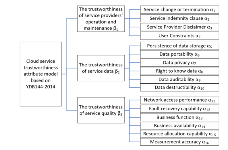
Figure 1: The cloud service-relevant reliability characteristic model [7].

Since Markov process is characterized by its memoryless property, the transitions between four trusted states \( {S_{1}},{S_{2}},{S_{3}},{S_{4}} \) can be predicted based on Markov chain principle by modeling a transition probability matrix. They represent a state of utmost trustworthiness, a fundamental assurance state, a crucial assurance state, and a doubted state, respectively [7]. The trusted state matrix is

\( TM=[\begin{matrix}Psi({S_{(1→1)}}) & Psi({S_{(1→2)}}) & Psi({S_{(1→3)}}) & Psi({S_{(1→4)}}) \\ Psi({S_{(2→1)}}) & Psi({S_{(2→2)}}) & Psi({S_{(2→3)}}) & Psi({S_{(2→4)}}) \\ Psi({S_{(3→1)}}) & Psi({S_{(3→2)}}) & Psi({S_{(3→3)}}) & Psi({S_{(3→4)}}) \\ Psi({S_{(4→1)}}) & Psi({S_{(4→2)}}) & Psi({S_{(4→3)}}) & Psi({S_{(4→4)}}) \\ \end{matrix}]\ \ \ (3) \)

where the element \( Psi({S_{m→n}}) \) is the probability of the reliability condition transforming from state \( m \) to state \( n \) , and \( \sum _{m=1}^{4}Psi({S_{(m→n)}})=1 \) .

3.1.2. Method of Computing the Reliable Condition of the Cloud Service

Expert evaluation of underlying indicators is that for each trusted attribute indicator \( {α_{j}} \) , experts evaluate its frequency level interval \( [{F_{min}}({α_{j}}),{F_{max}}({α_{j}})] \) , and the severity of loss level interval \( [{L_{min}}({α_{j}}),{L_{max}}({α_{j}})] \) .

Calculation of the Membership Degree \( {μ_{{S_{n}}}}({α_{j}}) \) is that the membership degree of the indicator \( {α_{j}} \) belong to state \( {S_{n}} \) is calculated by the geometric region overlapping method \( {μ_{{S_{n}}}}({α_{j}})=\frac{Square({α_{j}})∩Square({S_{n}})}{Square({α_{j}})} \) , where \( Square({α_{j}}) \) is the coverage area of \( {α_{j}} \) in the risk matrix, and \( Square({S_{n}}) \) is the geometric region of state \( {S_{n}} \) [7]. Calculation of Transition Probabilities by Integrating Membership Degrees is that for each trusted category \( {β_{i}} \) , the element \( P({S_{n}}→{S_{m}},{β_{i}}) \) of its transition matrix \( TM({β_{i}} ) \) is calculated by formula \( Psi({S_{n}}→{S_{m}},{β_{i}})=\sum _{j=1}^{total}{μ_{{S_{m}}}}({α_{j}}) \) when \( {μ_{{S_{n}}}}({α_{j}}) \gt 0 \) [7]. The trusted state matrix is given by

\( TM({β_{i}})=[\begin{matrix}Psi({S_{(1→1)}},{β_{i}}) & Psi({S_{(1→2)}},{β_{i}}) & Psi({S_{(1→3)}},{β_{i}}) & Psi({S_{(1→4)}},{β_{i}}) \\ Psi({S_{(2→1)}},{β_{i}}) & Psi({S_{(2→2)}},{β_{i}}) & Psi({S_{(2→3)}},{β_{i}}) & Psi({S_{(2→4)}},{β_{i}}) \\ Psi({S_{(3→1)}},{β_{i}}) & Psi({S_{(3→2)}},{β_{i}}) & Psi({S_{(3→3)}},{β_{i}}) & Psi({S_{(3→4)}},{β_{i}}) \\ Psi({S_{(4→1)}},{β_{i}}) & Psi({S_{(4→2)}},{β_{i}}) & Psi({S_{(4→3)}},{β_{i}}) & Psi({S_{(4→4)}},{β_{i}}) \\ \end{matrix}]\ \ \ (4) \)

Markov Chain Prediction: Suppose the probability vector of the trusted state at the current time \( t \) is \( {μ^{t}}=[μ_{{S_{1}}}^{t},μ_{{S_{2}}}^{t},μ_{{S_{3}}}^{t},μ_{{S_{4}}}^{t} ] \) , and the probability vector at the next moment is calculated by the transition matrix: \( {μ^{t+1}}={μ^{t}}∙TM({β_{i}}) \) [7].

In conclusion, this method quantifies uncertainties through fuzzy entropy and dynamically predicts state transitions using the Markov chain. It provides a systematic evaluation framework for the trustworthiness of cloud services from underlying indicators to global states, and is applicable to scenarios that require dynamic monitoring and risk prevention [7].

3.2. Markov Model for Predicting Network Traffic

3.2.1. Establishment of the Hidden Markov Model

In the immediate future, precise network traffic forecasts are essential for effective traffic management, which includes congestion reduction and traffic control [8]. For the foreseeable future, accurate network traffic forecasting will be crucial to the success of different traffic control techniques. However, because transportation systems are inherently unpredictable and chaotic, it can be difficult to achieve accurate forecasting in both free-flow and congested traffic conditions [8].

This paper showed a method that need to construct a hidden Markov model. The Hidden Markov Model, abbreviated as HMM, is a statistical model which is employed to depict a Markov process where there are hidden, unknown parameters [9]. It includes hidden states and observable states. The hidden states satisfy the Markov property, that is, the hidden state at the next moment depends only on the current hidden state and is independent of other historical states. Each hidden state will output an observable state with a certain probability [9]. HMM consists of observation set, which composed of all possible observation values; state transition probability matrix, which describes the probability of transitioning from one hidden step to another hidden step; and observation probability matrix, which represents the probability of generating each observation value under each hidden state [9]. In this case (prediction for network traffic), hidden states represent different levels or patterns of network activity, such as low traffic load, medium traffic load, and high traffic load states [8]. The observable states are the actual measurements of network traffic, which can be the number of packets transmitted per unit time [8]. The HMM attempts to classify the traffic fluctuations' results.

Construct a hidden Markov model with 3 hidden states \( {M_{1}},{M_{2}},{M_{3}} \) , which represents heavy traffic burden, moderate traffic burden and light traffic burden, respectively. The probability of transitioning between each state is based on the previous researches on specific observation states. As shown in the following matrix, where \( P \) stands for the matrix of concealed state transitions and \( π \) is the vector of original states probability [8]:

\( P=[\begin{matrix}P({M_{(1→1)}}) & P({M_{(1→2)}}) & P({M_{(1→3)}}) \\ P({M_{(2→1)}}) & P({M_{(2→2)}}) & P({M_{(2→3)}}) \\ P({M_{(3→1)}}) & P({M_{(3→2)}}) & P({M_{(3→3)}}) \\ \end{matrix}]\ \ \ (5) \)

\( π=[p({M_{1}}),p({M_{2}}),p({M_{3}})]\ \ \ (6) \)

If from state \( i \) transitions to state \( j \) occurs \( {N_{ij}} \) times, then \( {α_{ij}}=\frac{{N_{ij}}}{\sum _{k}{N_{ik}}} \) .

The calculating ways to predict the future states are shown in the follow. Using the transition matrix to iteratively compute future state distributions. For single-step prediction: the current state is \( {π_{t}} \) , then the next state distribution satisfies \( {π_{t+1}}={π_{t}}∙P \) [8]. For multi-step prediction: the future state \( {π_{t+k}} \) satisfies that \( {π_{t+k}}={π_{t}}∙{P^{k}} \) [8]. For example, if the observation state of the current state of the network traffic is "medium traffic load", that is, \( π=[0,1,0] \) . The transition matrix is \( P=[\begin{matrix}0.6 & 0.3 & 0.1 \\ 0.2 & 0.5 & 0.3 \\ 0.1 & 0.4 & 0.5 \\ \end{matrix}] \) . Therefore, the next state distribution is \( πP=[0.2,0.5,0.3] \) , that is, have 20% probability of “high traffic load”, 50% probability of “medium traffic load”, and 30% probability of “low traffic load”. For multi-step prediction, calculating \( {π_{t+k}}={π_{t}}∙{P^{k}} \) , as a result, \( {π_{t}} \) converges to \( [0.283,0.431,0.304] \) , satisfies the stationary distribution. Therefore, no matter what the conditions are, the probability of “high traffic burden” is 0.283, the probability of “medium traffic burden” is 0.431, and the probability of “low traffic burden” is 0.304.

3.2.2. Optimization: Training and Parameter Estimation of HMM

The Baum-Welch Algorithm (EM Algorithm) is shown as the follow. In E-step need to compute forward probability \( {α_{t}}(i)=P({x_{1}},{x_{2}},⋯,{x_{t}},⋯,{z_{t}}={q_{i}}) \) , which represents the joint probability that at time t, the state is \( {q_{i}} \) and the sequence \( {x_{1}},⋯,{x_{t}} \) has been observed. The backward probability \( {β_{t}}(i)=P({x_{t+1}},⋯,{x_{T}}|{z_{t}}={q_{i}}) \) , which represents the probability of observing the sequence \( {x_{t+1}},⋯,{x_{T}} \) given that the state at time \( t \) is \( {q_{i}} \) [8]. M-step is used to update the parameter \( P \) (the state-transition matrix), \( B \) (the observation probability matrix), and \( π \) (the original state probability vector) to maximize the likelihood function \( P(X)={π_{{Z_{1}}}}∙\prod _{t=1}^{T-1}{p_{{z_{t}}{z_{t+1}}}}∙\prod _{t=1}^{T}{b_{{z_{t}}}}({x_{t}}) \) , which describes the probability of the observed sequence \( X=({x_{1}},⋯,{x_{T}} ) \) occurring when given the parameters \( π \) , \( P \) , and \( B \) . By continuously adjusting \( π \) , \( P \) , and \( B \) , \( P(X) \) can increase [8].

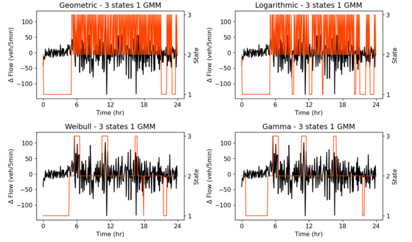
Figure 2: Determined hidden states based on varying sojourn densities, utilizing a model with 3 hidden states and incorporating 1 Gaussian mixture component [8].

Construction of Gaussian Mixture Model is \( {b_{j}}(x)=\sum _{l=1}^{k}{c_{jl}}N(x|{μ_{jl}},\sum _{jl}) \) , where \( k \) is the number of mixture components, \( {c_{jl}} \) is the weight of the \( l-th \) Gaussian component in the \( j-th \) state, and \( N(X|{μ_{jl}},\sum _{jl}) \) is the Gaussian distribution function with mean \( {μ_{jl}} \) and covariance \( \sum _{jl} [ \) 10]. As shown in Figure 2.

The overall goal is that after iteratively optimizing between the E-step and the W-step, the parameter combinations \( π \) , \( P \) , \( B \) and the parameters in Gaussian mixture model (if exist) that enhance the possibility to the likelihood of the observed data can be found to make the probability of the observed sequence occurring under the current parameters the largest [8]. One can then build up a multi-state dynamics model to capturing non-stationary through hidden states. In summary, the applications of hidden Markov model in modeling traffic by defining state and setting probability, estimating traffic by learning parameter, inferencing state and predicting traffic, and detecting anomaly by modeling normal patterns can help to better understand the patterns and dynamic changes of network traffic. They can also predict future traffic trends. As a result, it may enable human being to optimize the allocation of network resources, improve the quality of network services, and enhance network security protection.

4. Conclusion

In this paper, the author has explored the concepts and applications of Markov chains in computer science field. Citing the predictions of cloud service trusted state’s transformation and network traffic as two great examples, to show that with the great use of integrating Markov chain into some computation systems, training the systems by adapting the values of some important parameters, which were added into the Markov process, the future state can be predicted and then optimized. However, the limitations of this paper lie in lack of the support from some valid data and some computations of the operation of Markov process to verify the normal functioning of the systems.

In the future, Markov chain can also be used in the following fields of computer science. Such as in strengthening deep reinforcement learning by combing Markov chain with deep neural networks to handle sequential data with long-term dependencies, capture complex modes in time series more effectively, and improve the accuracy of the model's prediction of future states. This can be applied to multimodal tasks such as video analysis and speech recognition. In addition, in modeling the user's interaction behaviors in the virtual environment, such as the order and frequency of the user's interactions with virtual objects. Use Markov chains to generate more natural and user-habit-compliant interaction experiences, providing a basis for the design and optimization of the virtual environment. Overall, this paper may serve as a starting point for further investigations of Markov chain in computer science field.

References

[1]. Qian Zhiye, Li Xue & Li Suogang (2024). Efficient domain name generation algorithm based on improved Markov chain Journal of Communications (S2), 52-58
[2]. Chelly, I., Uziel, R., Freifeld, O., & Pakman, A. (2025). Consistent Amortized Clustering via Generative Flow Networks. arXiv preprint arXiv:2502.19337.
[3]. Li, J., Gibbons, R., & Rockova, V. (2025). Deep Computerized Adaptive Testing. arXiv preprint arXiv:2502.19275
[4]. Li, H., Xu, X., Peng, Y., & Chen, C. H. (2021). Efficient Sampling for Selecting Important Nodes in Random Network. IEEE Transactions on Automatic Control, 66(3), 1321–28.
[5]. Ross, S. M. (2014). Introduction to Probability Models. Netherlands: Academic Press.
[6]. Latifi, F., Nassiri, R., Mohsenzadeh, M., & Mostafaei, H. (2025). A Markov chain-based multi-criteria framework for dynamic cloud service selection using user feedback. The Journal of Supercomputing, 81(1), 89.
[7]. Yang, M., Jiang, R., Wang, J., Gui, B., & Long, L. (2024). Assessment of cloud service trusted state based on fuzzy entropy and Markov chain. Scientific Reports, 14(1), 1-18.
[8]. Sengupta, A., Das, A., & Guler, S. I. (2023). Hybrid hidden Markov LSTM for short-term traffic flow prediction. arXiv preprint arXiv:2307.04954.
[9]. H Weiß, C., & Swidan, O. (2024). Hidden-Markov models for ordinal time series. AStA Advances in Statistical Analysis, 1-23.
[10]. Saravanakumar, R., TamilSelvi, T., Pandey, D., Pandey, B. K., Mahajan, D. A., & Lelisho, M. E. (2024). Big data processing using hybrid Gaussian mixture model with salp swarm algorithm. Journal of Big Data, 11(1), 167.
Cite this article
Zhou,X. (2025). Applications of Markov Chain in the Field of Computer Science. Theoretical and Natural Science,100,149-156.
Data availability
The datasets used and/or analyzed during the current study will be available from the authors upon reasonable request.
Disclaimer/Publisher's Note
The statements, opinions and data contained in all publications are solely those of the individual author(s) and contributor(s) and not of EWA Publishing and/or the editor(s). EWA Publishing and/or the editor(s) disclaim responsibility for any injury to people or property resulting from any ideas, methods, instructions or products referred to in the content.
About volume
Volume title: Proceedings of the 3rd International Conference on Mathematical Physics and Computational Simulation
© 2024 by the author(s). Licensee EWA Publishing, Oxford, UK. This article is an open access article distributed under the terms and
conditions of the Creative Commons Attribution (CC BY) license. Authors who
publish this series agree to the following terms:
1. Authors retain copyright and grant the series right of first publication with the work simultaneously licensed under a Creative Commons
Attribution License that allows others to share the work with an acknowledgment of the work's authorship and initial publication in this
series.
2. Authors are able to enter into separate, additional contractual arrangements for the non-exclusive distribution of the series's published
version of the work (e.g., post it to an institutional repository or publish it in a book), with an acknowledgment of its initial
publication in this series.
3. Authors are permitted and encouraged to post their work online (e.g., in institutional repositories or on their website) prior to and
during the submission process, as it can lead to productive exchanges, as well as earlier and greater citation of published work (See
Open access policy for details).