1. Introduction

The accurate prediction of housing prices has always posed a significant challenge in the realm of quantitative real estate analysis. This complexity arises not only from the inherent spatial heterogeneity of real estate markets, such as location correlation and geographic spillovers, but also from the dynamic interplay of multiple socio-economic variables. These variables include population mobility, industrial agglomeration, and infrastructure networking. In order to systematically analyse these high-dimensional and non-linear relationships, regression analysis models can be constructed through parameter estimation from the perspective of mathematical modelling. This enables the quantification of the effects of explanatory variables on house prices. For complex dimensions, dimensionality reduction techniques such as Principal Component Analysis (PCA) can be introduced in order to effectively extract the essential features of the data or eliminate redundant information.

In the field of house price prediction, regression methods have been subject to extensive research and development. The proposal of the linear combination model provided the theoretical foundation for the subsequent development of traditional linear regression [1]. Subsequently, geostatistical techniques, such as Kriging, have emerged as a significant advancement [2,3]. The advent of the machine learning revolution has further enhanced predictive capabilities, with ensemble methods such as Artificial Neural Networks (ANN) [4], decision trees [5], Support Vector Machines (SVM) [5,6], and XGBoost [7,8] addressing nonlinear relationships and feature interactions. PCA is a core tool for the application of dimensionality reduction and feature extraction in house price prediction, as it can sometimes imporve the stability based on the hedonic model [9].

The study assesses the impact of PCA on three fundamental regression models (linear, ridge, and LASSO). Employing statistical validation (KMO test, Bartlett's test of sphericity) and interpretable component extraction, the study firstly achieves a dimensionality reduction of the data as a means of providing a high level overview of the main factors affecting regional house prices at the time and space scales in which they are located. In the subsequent phase, the analysis explores performance degradation mechanisms and theoretical contradictions.

2. Methodology

The dataset, sourced from Kaggle's California housing repository, presents a structured framework for predictive modeling with 20,640 observations and 10 covariates. Numeric variables exhibit two measurement scales: continuous (e.g., coordinates, income) and count data (e.g., rooms, population). The sole categorical variable Ocean Proximity contains five mutually exclusive classes: INLAND, <1H OCEAN, ISLAND, NEAR BAY, and NEAR OCEAN, requiring nominal encoding strategies for regression compatibility. Missing data occurs exclusively in Total Bedrooms (207 in total, approximately 1%). Significantly, Median House Value is considered as the target variable.

2.1. Problem Deconstruction and Preparation

The utilisation of regression analysis in the construction of house price prediction models constitutes a particularly valuable research option, primarily due to the fact that regression models provide clear parameter estimates.

The study will, at first, commence with the assumption that the target variable has a linear relationship with the other variables. Suppose that there are \( m \) samples and \( n \) original features for each sample. With the observed features, the original sample matrix and the design matrix can be, respectively, denoted as

\( {X_{orig}}=(\begin{matrix}\begin{matrix}{x_{11}} & {x_{12}} \\ {x_{21}} & {x_{22}} \\ \end{matrix} & \begin{matrix}⋯ & {x_{1n}} \\ ⋯ & {x_{2n}} \\ \end{matrix} \\ \begin{matrix}⋮ & ⋮ \\ {x_{m1}} & {x_{m2}} \\ \end{matrix} & \begin{matrix}⋱ & ⋮ \\ ⋯ & {x_{mn}} \\ \end{matrix} \\ \end{matrix}), {X_{design}}=(\begin{matrix}\begin{matrix}1 & {x_{11}} \\ 1 & {x_{21}} \\ \end{matrix} & \begin{matrix}{x_{12}} & ⋯ & {x_{1n}} \\ {x_{22}} & ⋯ & {x_{2n}} \\ \end{matrix} \\ \begin{matrix}⋮ & ⋮ \\ 1 & {x_{m1}} \\ \end{matrix} & \begin{matrix}⋮ & ⋱ & ⋮ \\ {x_{m2}} & ⋯ & {x_{mn}} \\ \end{matrix} \\ \end{matrix}) \) .

Following the implementation of PCA, the original n features of each sample are obtained as \( N \) principal components, which are denoted by \( {z_{1}},{z_{2}},⋯,{z_{N}} \) . Then, a new sample matrix and a new design matrix of can be obtained from:

\( {X_{PCA}}=(\begin{matrix}\begin{matrix}{z_{11}} & {z_{12}} \\ {z_{21}} & {z_{22}} \\ \end{matrix} & \begin{matrix}⋯ & {z_{1N}} \\ ⋯ & {z_{2N}} \\ \end{matrix} \\ \begin{matrix}⋮ & ⋮ \\ {z_{m1}} & {z_{m2}} \\ \end{matrix} & \begin{matrix}⋱ & ⋮ \\ ⋯ & {z_{mN}} \\ \end{matrix} \\ \end{matrix}), {X_{design-PCA}}=(\begin{matrix}\begin{matrix}1 & {z_{11}} \\ 1 & {z_{21}} \\ \end{matrix} & \begin{matrix}{z_{12}} & ⋯ & {z_{1N}} \\ {z_{22}} & ⋯ & {z_{2N}} \\ \end{matrix} \\ \begin{matrix}⋮ & ⋮ \\ 1 & {z_{m1}} \\ \end{matrix} & \begin{matrix}⋮ & ⋱ & ⋮ \\ {z_{m2}} & ⋯ & {z_{mN}} \\ \end{matrix} \\ \end{matrix}). \)

The standardisation is applied to the sample matrices in order to eliminate quantitative differences and order-of-magnitude inconsistencies between the features. For the sake of simplicity and convenience, the standardised matrices are labelled with the same notations.

For each sample \( i (i=1,2,3,⋯,m) \) , the observed Median House Value as the variable of interest is denoted as \( {p_{i}} \) . Technically, the assumption above enables the regression coefficients to be utilised to create a linear combination of each original attribute or principal component element and the intercept term. Thus, for the target variable, the regression coefficients and feature coefficients, they can be tabulated respectively as

\( P=(\begin{matrix}\begin{matrix}{p_{1}} \\ {p_{2}} \\ \end{matrix} \\ \begin{matrix}⋮ \\ {p_{m}} \\ \end{matrix} \\ \end{matrix}), β=(\begin{matrix}\begin{matrix}{β_{0}} \\ {β_{1}} \\ \end{matrix} \\ \begin{matrix}{β_{2}} \\ ⋮ \\ {β_{N}} \\ \end{matrix} \\ \end{matrix}),{β_{feat}}=(\begin{matrix}{β_{1}} \\ \begin{matrix}{β_{2}} \\ ⋮ \\ {β_{N}} \\ \end{matrix} \\ \end{matrix}). \)

2.2. Extraction and Interpretation of Principal Components

In property market analysis, house price prediction is challenged by complex interrelated factors, necessitating dimensionality reduction to mitigate modeling complexity. This study employs Principal Component Analysis (PCA) to extract uncorrelated composite indicators while preserving data integrity. Plus, the joint utilisation of KMO and Bartlett's test before PCA is imperative and valid [10].

2.3. Construction of Regression Models

This study constructs four distinct regression analysis model frameworks. During the data preprocessing phase, missing value imputation and one-hot encoding methods are employed to ensure data quality, followed by partitioning the dataset into training and test sets to enhance model robustness. Parameters of models (ridge regression, LASSO regression, PLSR) are manually preset and subsequently trained on the training set. Finally, the performance of the models was systematically validated using multi-dimensional evaluation metrics on the test set.

2.3.1. Multiple Linear Regression (MLR)

MLR models the relationship between the target variable and features by minimizing the residual sum of squares. For the original features (PCA-unprocessed), the model assumes

\( P={X_{design}}β+ε, \)

and the closed-form solution is

\( {β_{OLS}}={(X_{design}^{T}{X_{design}})^{-1}}X_{design}^{T}P. \)

After PCA, the solution adapts to

\( {β_{OLS}}={(X_{design-PCA}^{T}{X_{design-PCA}})^{-1}}X_{design-PCA}^{T}P. \)

2.3.2. LASSO Regression

LASSO regression introduces \( {L_{1}} \) -regularization to promote sparsity in feature coefficients. For the original features, the objective is

\( {min_{β}}‖P-{X_{design}}β‖_{2}^{2}+α{‖{β_{feat}}‖_{1}}. \)

After PCA, the regularization applies to principal components:

\( {min_{β}}‖P-{X_{design-PCA}}β‖_{2}^{2}+α{‖{β_{feat}}‖_{1}}. \)

The solution remains numerical (e.g., coordinate descent) where \( α=0.1 \) in the study case.

2.3.3. Ridge Regression

Ridge regression employs \( {L_{2}} \) -regularization to shrink coefficients and handle multicollinearity. Using original features, the objective is

\( {min_{β}}‖P-{X_{design}}β‖_{2}^{2}+λ‖{β_{feat}}‖_{2}^{2}, \)

with closed-form solution

\( {β_{ridge}}={(X_{design}^{T}{X_{design}}+λI)^{-1}}X_{design}^{T}P. \)

After PCA, the regularization operates on principal components:

\( {β_{ridge}}={(X_{design-PCA}^{T}{X_{design-PCA}}+λI)^{-1}}X_{design-PCA}^{T}P. \)

And \( λ=1 \) as the preset parameter.

3. Results

3.1. Results of Principal Components Extraction

The KMO test results reveal critical limitations in the suitability of the variable Ocean Proximity for principal component analysis. With an overall KMO value below the recommended threshold of 0.5, this variable demonstrates inadequate sampling adequacy for factor extraction. Notably, only the “NEAR BAY” subcategory marginally exceeds this criterion (KMO > 0.6) [11], while all other subcategories fall below 0.5. This statistical evidence indicates weak partial correlations between Ocean Proximity and other variables in the dataset, compromising its analytical value in multivariate dimensionality reduction. However, a substantive decision was made to exclude this variable from subsequent PCA procedures based on geographical rationality.

Table 1:KMO Values for Different Ocean Proximity Categories

Table 2: Final Results of KMO Test and Bartlett's Test.

(Note: *** indicates significance at the 1% level.)

Subsequently, the KMO test and Bartlett's test of sphericity are conducted once more on the residual numerical variables. This results in the acquisition of novel outcomes, exhibiting elevated KMO values (> 0.6). This signifies that the data are more appropriate for PCA analysis than previously determined. The decision to perform PCA is further supported by the significant Bartlett test result (p < 0.05) [12].

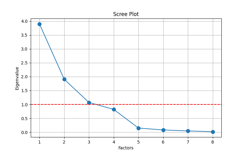
Figure 1: Scree Plot for Factor Analysis.

Principal component extraction combined methodological validation: the Elbow Method [13] identified three components at the scree plot inflection point, while the Kaiser Criterion [14] theoretically supported this selection.

The principal component interpretation in Table 3 reveals distinct thematic dimensions [15]. In Table 3, PC1 exhibits dominant loadings (>0.9) on Total Rooms, Total Bedrooms, Population, and Households, thereby operationalizing the latent construct ‘Spatial Distribution & Density’. PC2 derives from longitudinal and latitudinal coordinates (factor loadings ±0.9), substantiating its designation as ‘Geographic Location’ through geospatial data alignment. PC3 demonstrates selective sensitivity to Median Income (loading 0.996), establishing its validity as the ‘Economic Status’ indicator. This nomenclature system maintains interpretive coherence with both statistical loadings and theoretical expectations, while component loadings exceeding |0.5| threshold across all retained factors validate variable-group conceptual integration.

Table 3: Component Loadings for PCA.

3.2. Performance Analysis

The following section presents the findings derived from the application of the regression models to the specified dataset, and provides a comprehensive summary of the comparison of these models.

In the study, all models demonstrated a significant linear trend, irrespective of the implementation of PCA treatment. In Table 4, the fitted slopes of linear regression, ridge regression and LASSO based on the original data were stable around 0.649, indicating that the original features can effectively capture about 65% of the house price fluctuation information. Regression analyses conducted through the three principal components after PCA treatment revealed that the slopes of each model produced a similar degree of change, with all model slopes uniformly decreasing to the range of 0.4678 — a decrease of 28% — and the differences in slopes across models narrowed to the order of 10^-5.

Table 4: Fitting Effect Slopes of Different Regression Methods Before and After PCA.

In Figure 2, the original models obtained prior to PCA demonstrated a superior capacity to capture changing trends, with their overall trends exhibiting a closer alignment with the ideal state. Furthermore, Figure 2 reveals that the intersection points of the three curves under each model are highly proximate, suggesting that each model exhibits a superior predictive accuracy within the image’s central region.

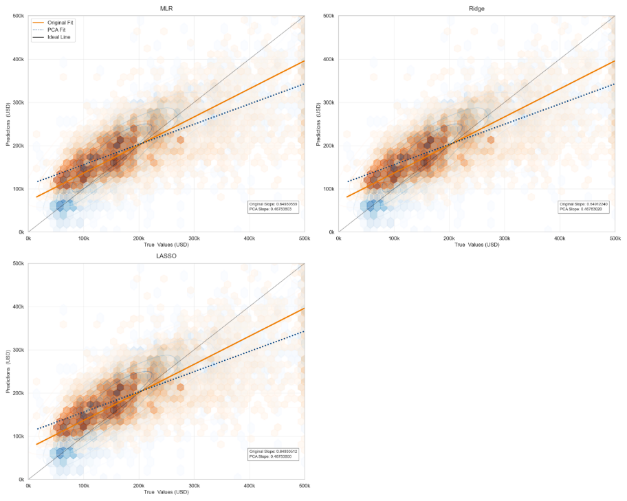
Figure 2: True vs. Predicted Plot

The cross-sectional comparison of different models under the same dataset demonstrates that PCA has a detrimental effect on model prediction under these conditions. Furthermore, the longitudinal comparison of the same model before and after PCA reveals that PCA results in a decline in performance.

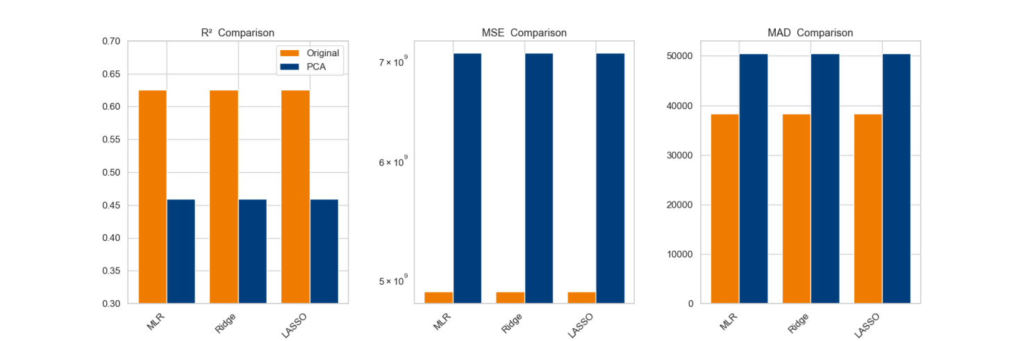
Figure 3: Performance Comparison.

In Figure 3, it is evident that, after the incorporation of PCA, the three models demonstrated a reduction in their explanatory capacity regarding data variability, concurrently accompanied by systematic amplification of prediction errors and diminished robustness. R² quantifies the proportion of dependent variable variance explained by the model, reflecting regression goodness-of-fit. The R² values of all models were elevated when the original dataset was employed directly for prediction, where linear regression, ridge regression and LASSO regression demonstrating particular efficacy. Conversely, the R² values of the models appeared to decline following PCA. MSE measures the average squared deviation between predicted and true values. In this study, the comparison of MSE revealed that the errors in the original dataset were generally low, and that there was a significant increase in errors after PCA. MAD evaluates prediction accuracy via mean absolute deviations. The embodied MAD of the regression models were partially increased via PCA, and the improvement was not significant.

To be more precise, the R² of linear regression, ridge regression, and LASSO regression were all approximately 0.626, suggesting comparable performance. Following PCA, the original attributes were converted to orthogonal principal components, thereby theoretically eliminating the covariance. However, the R² of all models was 0.459, indicating that the principal components lost some key information. The comparison of the regression performance of the same models before and after PCA reveals that the principal components failed to fully retain information related to house prices.

4. Discussions & Conclusions

The study proposes an initial and elemental ‘spatial-economic-social’ framework when investigating house price impacts, with the concern that PCA orthogonalization attenuates regularization efficacy.

The PCA reveals three primary components that exert significant influence: ‘Spatial Distribution & Density’, ‘Geographic Location’ and ‘Economic Status’. These components offer a concise summary of the factors influencing house prices in the region, including house type, population, geographic location and economic factors. This finding aligns with the observations derived from the variable intuition approach. Consequently, this underscores the notion that house prices are not determined by a solitary factor but are shaped through multidimensional interactions within the spatial economic system. The three principal components obtained in this study facilitate the comprehension of the intricate mechanism of urban house price formation as a straightforward ‘spatial-economic-social’ three-dimensional synergistic influencing framework, where alterations in any of these dimensions are transmitted to the housing market through a comparable linear effect within a specified time and space horizon.

Notwithstanding, in the case study, there is seemingly few improvement for performances after PCA, even with regularization in LASSO model and Ridge model. It is noteworthy that the PCA orthogonalisation satisfies \( X_{orig}^{T}{X_{orig}}=I \) which changes the mechanism of action of regularisation. More significantly, the OLS estimation is

\( {β_{OLS}}=X_{design-PCA}^{T}P, \)

and the ridge regression degenerates to isotropic shrinkage:

\( {β_{ridge}}={(X_{design-PCA}^{T}{X_{design-PCA}}+λI)^{-1}}X_{design-PCA}^{T}P=\frac{1}{1+λ}{β_{OLS}}, \)

In orthogonalized feature spaces, collinear features are decorrelated, causing \( {L_{2}} \) -regularization to lose its directional sensitivity. The penalty term reduces to axis-aligned scaling, forfeiting its capacity to differentially shrink coefficients based on data geometry. In actual, when principal components with high-variance exhibit weak contributions to Y, while low-variance components demonstrate substantial predictive power, uniform shrinkage mechanisms disproportionately suppress critical features, thereby amplifying estimation bias and degrading model performance, and all coefficients in the study are uniformly scaled by \( \frac{1}{(1+λ)} \) , explaining why ridge and OLS metrics are nearly identical. Equally critical is that LASSO reduces to soft-thresholded OLS in orthogonal space. The LASSO problem decouples into \( N \) independent univariate optimizations:

\( {min_{{β_{j}}}}{({β_{j}}-{β_{OLS,j}})^{2}}+α|{β_{j}}|, where j≥1. \)

By taking derivative and solving for \( {β_{j}} \) , one can obtain

\( {β_{j}}=sign({β_{OLS,j}})\cdot {({β_{OLS,j}}-\frac{α}{2})_{+}}, \)

where \( {(x)_{+}}=max(x,0) \) , shrinking small coefficients to zero. Thus, in this study, \( α \) was too small to induce sparsity, making the improvement so faint.

In conclusion, while PCA can simplify the model to a certain extent, in this study, PCA is more valuable in highlighting the main factors affecting regional house prices in that spatio-temporal range from the dimension of the data. Furthermore, the enhancement of ridge regression and LASSO regression for MLR based on linear assumptions is not significant. In the context of the deep penetration of intelligent data analytics into the real estate sector, it is suggested that PCA with regression analysis alone carries some potential risks, and that PCA may no longer be the default preprocessing step. It is recommended that PCA be adopted with caution and with consideration of a domain-specific regularisation strategy to balance interpretability and prediction fidelity.

References

[1]. Rosen, S. (1974). Hedonic prices and implicit markets: Product differentiation in pure competition. Journal of Political Economy, 82(1), 34–55. https://doi.org/10.1086/260169
[2]. de Koning, K., Filatova, T., & Bin, O. (2018). Improved methods for predicting property prices in hazard prone dynamic markets. Environmental & Resource Economics, 69(2), 247–263. https://doi.org/10.1007/s10640-016-0076-5
[3]. Chica-Olmo, J., Cano-Guervos, R., & Tamaris-Turizo, I. (2019). Determination of buffer zone for negative externalities: Effect on housing prices. Geographical Journal, 185(2), 222–236. https://doi.org/10.1111/geoj.12289
[4]. Alzain, E., Alshebami, A. S., Aldhyani, T. H. H., & Alsubari, S. N. (2022). Application of artificial intelligence for predicting real estate prices: The case of Saudi Arabia. Electronics, 11(21), 3448. https://doi.org/10.3390/electronics11213448
[5]. Soltani, A., Heydari, M., Aghaei, F., & Pettit, C. J. (2022). Housing price prediction incorporating spatio-temporal dependency into machine learning algorithms. Cities, 131, 103941. https://doi.org/10.1016/j.cities.2022.103941
[6]. Akyuz, S. Ö., Erdogan, B. E., Yildiz, Ö., & Atas, P. K. (2023). A novel hybrid house price prediction model. Computational Economics, 62(3), 1215–1232. https://doi.org/10.1007/s10614-022-10298-8
[7]. Arancibia, R. G., Llop, P., & Lovatto, M. (2023). Nonparametric prediction for univariate spatial data: Methods and applications. Papers in Regional Science, 102(3), 635. https://doi.org/10.1111/pirs.12735
[8]. Zhan, C., Liu, Y., Wu, Z., Zhao, M., & Chow, T. W. S. (2023). A hybrid machine learning framework for forecasting house price. Expert Systems with Applications, 233, 120981. https://doi.org/10.1016/j.eswa.2023.120981
[9]. Jolliffe, I. T., & Cadima, J. (2016). Principal component analysis: A review and recent developments. Philosophical Transactions of the Royal Society A: Mathematical, Physical and Engineering Sciences, 374(2065), 20150202. https://doi.org/10.1098/rsta.2015.0202
[10]. Costello, A. B., & Osborne, J. W. (2005). Best practices in exploratory factor analysis: Four recommendations for getting the most from your analysis. Practical Assessment, Research and Evaluation, 10(7).
[11]. Kaiser, H. F. (1974). An index of factorial simplicity. Psychometrika, 39(1), 31–36. https://doi.org/10.1007/BF02291575
[12]. Bartlett, M. S. (1950). Tests of significance in factor analysis. British Journal of Psychology - Statistical Section, 3(2), 77–85. https://doi.org/10.1111/j.2044-8317.1950.tb00285.x
[13]. Cattell, R. B. (1966). Scree test for number of factors. Multivariate Behavioral Research, 1(2), 245–276. https://doi.org/10.1207/s15327906mbr0102_10
[14]. Kaiser, H. F. (1960). The application of electronic computers to factor analysis. Educational and Psychological Measurement, 20(1), 141–151. https://doi.org/10.1177/001316446002000116
[15]. Jolliffe, I. T. (1986). Principal component analysis (Springer series in statistics). Springer-Verlag. https://doi.org/10.1007/978-1-4757-1904-8
Cite this article
Xiong,T. (2025). Dimensionality-Prediction Dilemma: The Dual Effects of PCA in Housing Price Regression Modeling. Theoretical and Natural Science,100,204-212.
Data availability
The datasets used and/or analyzed during the current study will be available from the authors upon reasonable request.
Disclaimer/Publisher's Note
The statements, opinions and data contained in all publications are solely those of the individual author(s) and contributor(s) and not of EWA Publishing and/or the editor(s). EWA Publishing and/or the editor(s) disclaim responsibility for any injury to people or property resulting from any ideas, methods, instructions or products referred to in the content.
About volume
Volume title: Proceedings of the 3rd International Conference on Mathematical Physics and Computational Simulation
© 2024 by the author(s). Licensee EWA Publishing, Oxford, UK. This article is an open access article distributed under the terms and
conditions of the Creative Commons Attribution (CC BY) license. Authors who
publish this series agree to the following terms:
1. Authors retain copyright and grant the series right of first publication with the work simultaneously licensed under a Creative Commons
Attribution License that allows others to share the work with an acknowledgment of the work's authorship and initial publication in this
series.
2. Authors are able to enter into separate, additional contractual arrangements for the non-exclusive distribution of the series's published
version of the work (e.g., post it to an institutional repository or publish it in a book), with an acknowledgment of its initial
publication in this series.
3. Authors are permitted and encouraged to post their work online (e.g., in institutional repositories or on their website) prior to and
during the submission process, as it can lead to productive exchanges, as well as earlier and greater citation of published work (See
Open access policy for details).