1. Introduction

In the field of modern signal processing, the issue of signal denoising has always been an important research topic. With the continuous development of information technology and communication systems, the impact of noise pollution on signal quality has become more severe, particularly in fields such as wireless communication, audio processing, and medical imaging. The challenge of efficiently removing noise and improving signal quality has become urgent. Especially in complex and dynamically changing noisy environments, traditional denoising methods are often constrained by various factors, resulting in unsatisfactory denoising performance. Therefore, designing an efficient denoising algorithm capable of adapting to different noise characteristics has become a hot topic in signal processing.

Adaptive filtering algorithms [1-3] have demonstrated substantial efficacy in signal denoising, attributable to their capability to dynamically adjust filter parameters in real time and accommodate environmental variations. The Least Mean Squares (LMS) [4] and Normalized Least Mean Squares (NLMS) [2,5] algorithms, as classic adaptive algorithms, have performed excellently in many applications. Due to its simplicity and real-time capability, the LMS algorithm is widely used in noise removal. However, the LMS algorithm has limitations in convergence speed and performance, especially in cases where the noise is complex and unstable. The algorithm exhibits a gradual convergence rate, resulting in a constrained denoising efficacy. To mitigate this issue, researchers have proposed enhanced algorithms, including NLMS and Recursive Least Squares (RLS), which optimize the performance of the LMS algorithm through the incorporation of alternative updating mechanisms and parameter adjustment methodologies. However, these algorithms still face challenges when dealing with complex signals such as non-Gaussian noise and long-tailed noise.

Currently, adaptive filtering algorithms based on statistical methods, especially those that use second-order statistics (SOS) [6,7] to estimate signal characteristics, have become a hot research topic. Compared to traditional methods, the SOS method can more effectively capture the noise features in the signal, thereby improving the denoising performance. However, despite extensive research in this direction, how to fully leverage the advantages of SOS in various noisy environments remains an open issue. Additionally, although existing adaptive algorithms have shown good results in theoretical analyses, problems such as computational complexity, real-time performance, and stability have not been adequately addressed in practical applications.

Therefore, this study aims to fill this gap by proposing an improved adaptive filtering algorithm based on second-order statistics. The performance of the algorithm will be evaluated in various noisy environments, and its advantages and practical feasibility will be verified through simulation analysis. Through systematic comparison and optimization, this study aims to develop a more efficient and adaptable algorithm for signal denoising, thereby advancing the application of adaptive filtering technology in complex signal processing scenarios.

2. Design and Optimization of Adaptive Filtering Algorithms

2.1. Principle of Adaptive Filtering

Adaptive filtering is a technique that dynamically adjusts filter coefficients to accommodate changes in signal characteristics. It is widely used in areas such as speech denoising, echo cancellation, and channel equalization. In speech denoising, adaptive filtering leverages the statistical properties of both noise and speech signals to adjust the filter parameters in real time, effectively suppressing background noise while preserving the clarity of the speech signal.

The block diagram of the principle of an adaptive filter is shown in Figure 1. The input signal x(n) is passed through a parameter-adjustable digital filter to produce the output signal y(n), which is then compared with the desired signal d(n) to generate the error signal e(n) The filter parameters are adjusted through the adaptive algorithm to minimize the mean square value of e(n).Adaptive filtering can utilize the results of previously obtained filter parameters to automatically adjust the filter parameters at the current time, adapting to unknown or time-varying statistical properties of the signal and noise, thus achieving optimal filtering. An adaptive filter is essentially a Wiener filter that adjusts its own transmission characteristics to achieve optimal performance. It does not require prior knowledge of the input signal, has low computational complexity, and is particularly suitable for real-time processing. Wiener filter parameters are fixed and suitable for stationary random signals, while Kalman filter parameters are time-varying and suitable for non-stationary random signals. However, these two filtering techniques can only achieve optimal filtering when the statistical properties of the signal and noise are known in advance. In practical scenarios, acquiring prior knowledge of the statistical properties of both the signal and noise is frequently infeasible. Under these circumstances, adaptive filtering techniques can deliver superior filtering performance, thereby rendering them exceptionally valuable in real-world applications.

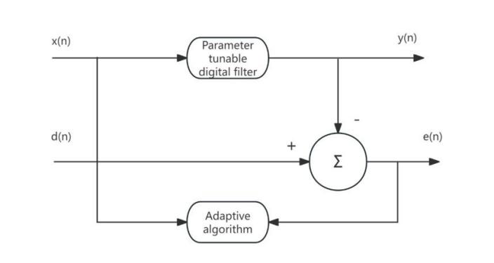
Figure 1: Block diagram of adaptive filter

The input signal vector:

\( x(n)={[x(n)x(n-1)…x(n-L)]^{T}}\ \ \ (1) \)

The output \( y(n) \) is:

\( y(n)=\sum _{k=0}^{L}{w_{k}}(n)x(n-k)\ \ \ (2) \)

The \( L+1 \) weight coefficients of the adaptive linear combiner form a weight coefficient vector, referred to as the weight vector, denoted as \( w(n) \) , i.e.,

\( w(n)={[{w_{0}}(n){w_{1}}(n)…{w_{L}}(n)]^{T}}\ \ \ (3) \)

Therefore, \( y(n) \) can be expressed as:

\( y(n)={x^{T}}(n)w(n)={w^{T}}(n)x(n)\ \ \ (4) \)

The error signal is:

\( e(n)=d(n)-y(n)=d(n)-{x^{T}}(n)w(n)=d(n)-{w^{T}}(n)x(n)\ \ \ (5) \)

The adaptive linear combiner follows the criterion of minimizing the mean square value of the error signal, i.e.,

\( ξ(n)=E[{e^{2}}(n)]=E[{d^{2}}(n)]+{w^{T}}(n)E[x(n){x^{T}}(n)]w(n)-2E[d(n){x^{T}}(n)]w(n)\ \ \ (6) \)

The autocorrelation matrix of the input signal is:

\( \begin{array}{c} R=E[x(n){x^{T}}(n)] \\ =[ \begin{array}{c} E[x(n)x(n)]E[x(n)x(n-1)]…E[x(n)x(n-L)] \\ E[x(n-1)x(n)]E[x(n-1)x(n-1)]…E[x(n-1)x(n-L)] \\ E[x(n-L)x(n)]E[x(n-L)x(n-1)]…E[x(n-L)x(n-L)] \end{array} ] \end{array} \ \ \ (7) \)

The cross-correlation matrix of the desired signal and the input signal is:

\( \begin{array}{c} P=E[d(n)x(n)] \\ =E[d(n)x(n)d(n)x(n-1)…d(n)x(n-L)] \end{array} \ \ \ (8) \)

The simple expression of the mean square error is:

\( ξ(n)=E[{d^{2}}(n)]+{w^{T}}Rw-2{P^{T}}w\ \ \ (9) \)

From this equation, it can be observed that under the assumption that both the input signal and the reference response are stationary random signals, the mean square error is a quadratic function of the components of the weight vector. The graph of this function is a hyperparaboloid in an L+2-dimensional space, with a unique minimum point. This surface is called the mean square error performance surface, or simply the performance surface.

The gradient of the mean square error performance surface:

\( ∇=\frac{∂w}{∂ξ}=2Rw-2P\ \ \ (10) \)

Setting the gradient to zero yields the optimal weight vector, or Wiener solution, corresponding to the minimum mean square error, which is derived as follows:

\( {w^{*}}={R^{-1}}P\ \ \ (11) \)

Although the expression for the Wiener solution is known in this paper, several issues remain:

a. It is necessary to know R and P, but both of these are unknown in this paper a priori;

b. The computational cost of the matrix inversion is too high: \( O(n³) \) ;

c. If the signal is non-stationary, R and P vary each time, requiring repeated computations.

2.2. Optimization of Adaptive Filtering

Based on the existing LMS and NLMS algorithms, this paper proposes an adaptive filtering algorithm that incorporates second-order statistics (SOS). This algorithm is particularly employed for signal denoising in high-noise environments, effectively enhancing both the convergence speed and denoising accuracy of the filter.

a.Signal Model

Suppose the input signal consists of a useful signal \( s(n) \) and noise \( w(n) \) , i.e.,

\( x(n)=s(n)+w(n)\ \ \ (12) \)

Here, x(n) is the noisy signal, \( s(n) \) is the true signal, and \( w(n) \) is the noise.

b. Adaptive Filter

The adaptive filter \( s(n) \) is used to process the signal. The output of the filter is an estimate of the true signal:

\( \hat{s}(n)={w^{T}}(n)x(n)\ \ \ (13) \)

Here, \( w(n) \) is the weight vector of the filter, and \( x(n) \) is the input vector.

c. Error Signal: The error is defined as the difference between the filter output and the true signal:

\( e(n)=s(n)-\hat{s}(n)\ \ \ (14) \)

d. Second-Order Statistics (SOS): To accelerate the convergence speed and improve denoising accuracy, this paper incorporates the second-order statistical properties of the input signal. The covariance matrix of the input signal is considered when updating the filter weights:

\( R=E[x(n){x^{T}}(n)]\ \ \ (15) \)

This matrix is used to accelerate the update of the filter parameters.

e. Weight Update Formula: In the traditional LMS algorithm, the weight update formula is:

\( w(n)=w(n-1)+μx(n)e(n)\ \ \ (16) \)

In the improved algorithm presented in this paper, second-order statistics are incorporated, resulting in the following update formula:

\( w(n)=w(n-1)+μ{R^{-1}}x(n)e(n)\ \ \ (17) \)

Here, \( {R^{-1}} \) is the inverse of the input signal’s covariance matrix, and μ is the step size.

3. Noise Modeling and Characteristic Analysis

3.1. Noise Modeling

Due to the wide variety of noise types and characteristics, it is necessary to establish appropriate noise models based on specific application scenarios. This paper will discuss several common types of noise and their modeling methods, including Gaussian noise, non-Gaussian noise, and heavy-tailed noise, among others [1,2].

Gaussian noise is the most common type of noise, and it is typically assumed that the noise distribution follows a normal distribution. The characteristics of Gaussian noise include a mean of zero and a constant variance, with its probability density function forming a bell-shaped curve. The advantage of Gaussian noise lies in its simplicity, as it can be well represented by the mean and variance parameters. In many signal processing applications, especially in communication systems and image processing, Gaussian noise serves as the standard noise model. To more accurately model noise in practical applications, this paper will examine statistical characteristics including the noise’s covariance matrix and autocorrelation function, thereby establishing a theoretical foundation for subsequent denoising algorithms.

Non-Gaussian noise refers to noise types that do not follow a normal distribution, such as impulse noise, speckle noise, etc. The statistical characteristics of non-Gaussian noise are often more complex and may exhibit asymmetry, spikes, or heavy-tailed distributions. Given that the distribution of these noises deviates from Gaussian noise, traditional denoising methods reliant on Gaussian assumptions frequently fail to effectively eliminate such noise. To accurately model non-Gaussian noise, this paper incorporates higher-order statistics or employs mixture distribution models, thereby more precisely capturing the actual behavior of the noise.

Heavy-tailed noise refers to noise whose probability distribution has a thicker tail, meaning that the probability near extreme values is higher. It is commonly seen in fields such as financial data and interference in communication signals. Heavy-tailed noise often exhibits self-similarity and heavy-tail characteristics, making it difficult for traditional Gaussian noise models to capture its features. When modeling heavy-tailed noise, stable distributions, Cauchy distributions, and other probability distributions characterized by heavy tails are typically utilized to describe its statistical properties. Modeling heavy-tailed noise is crucial for the design of denoising algorithms, as it helps the algorithm more effectively handle extreme values in the noise.

3.2. Noise Characteristic Analysis

The second-order moment characteristics of noise (such as mean, variance, and autocorrelation function) play an important role in noise identification and removal. This paper will focus on analyzing the second-order moment characteristics of noise and explore the application of second-order statistics in noise identification and removal.

The second-order moment characteristics of noise mainly include the mean, variance, and autocorrelation function. The mean reflects the average level of the noise, the variance describes the fluctuation degree of the noise, and the autocorrelation function reveals the correlation of the noise at different time or spatial locations. For Gaussian noise, the second-order moment characteristics are relatively simple and can usually be fully described by the mean and variance. However, for non-Gaussian and heavy-tailed noises, second-order moment characteristics are often insufficient to fully describe their features. In such cases, higher-order statistics or more complex noise models need to be introduced for accurate modeling.

Second-order statistics (such as the noise's autocorrelation function and covariance matrix) play an important role in noise identification. By calculating these statistics, this paper can identify the type, strength, and time-domain and frequency-domain characteristics of the noise. For instance, in certain applications, the noise may manifest periodic or abrupt jump characteristics, which can be effectively discerned through the autocorrelation function, thereby providing valuable insights for noise removal. The results of noise identification can further guide the design of denoising algorithms, helping to choose the appropriate filter or denoising method.

In noise removal, second-order statistics can help optimize filter design and improve denoising performance. For example, in adaptive filtering, the noise's autocorrelation function can be used to design more precise filters, making them more effective in removing noise in complex noise environments. Furthermore, second-order statistics can be harnessed to dynamically adjust denoising strategies, enabling the filter to adapt to varying types of noise and their fluctuations. By leveraging the second-order moment characteristics of the noise, denoising algorithms can sustain robust performance across diverse noise environments, particularly in scenarios characterized by non-Gaussian or heavy-tailed noise characteristics.

4. Simulation Experiments and Performance Analysis

4.1. Simulation Experiments

To verify the effectiveness of the proposed second-order statistics-based adaptive filtering algorithm, this study will conduct a series of simulation experiments in the MATLAB environment. The main objective of the simulation experiments is to evaluate the algorithm's performance in practical applications by simulating different types of noise and signal conditions. Various noise types, such as Gaussian noise, non-Gaussian noise, and heavy-tailed noise, will be used in the simulation experiments. The signal sources will include different types of test signals, such as sine waves, random noise signals, and actual data sequences.

In the experimental design, this study will compare the performance of classical adaptive filtering algorithms (such as LMS and NLMS) with the proposed second-order statistics-based adaptive filtering algorithm. Each algorithm will be run under the same noise conditions and its performance will be comprehensively evaluated using multiple metrics.

The simulation process will simulate the transmission and filtering of signals under different noise conditions, gradually observing the quality of the filtered output signal. Specifically, this study will focus on the differences between algorithms in terms of denoising effectiveness, stability, adaptability, and convergence under high-noise environments.

First, this study will apply the LMS and NLMS algorithms to filter the same PPG signal, yielding the original and filtered PPG signals shown in Figures 2 and 3, respectively.

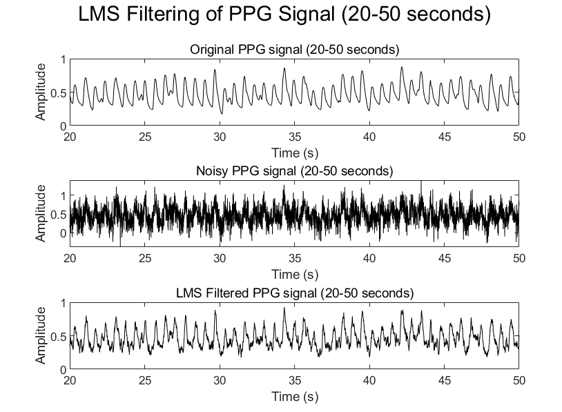
Figure 2: PPG signal filtered by LMS algorithm(20-50seconds)

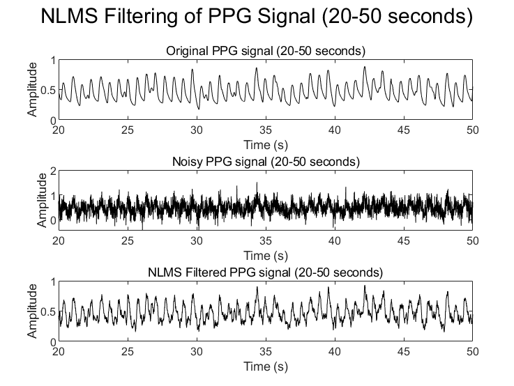
Figure 3: PPG signal filtered by NLMS algorithm(20-50seconds)

Next, the proposed algorithm will be used to filter the same PPG signal, resulting in the signal shown in the figure below.

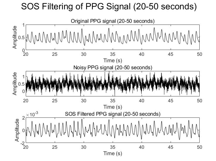
Figure 4: PPG signal filtered by SOS algorithm(20-50seconds)

As illustrated in Figure 4, the salient advantage of this algorithm is its ability to obviate the need for stepwise weight adjustment, instead directly computing through covariance and variance, thereby offering a solution that is both simple and intuitive. In contrast, the LMS algorithm necessitates iterative weight updates, whereas the second-order statistics method accomplishes the calculation in a single step. The LMS algorithm is sensitive to the step size parameter, while the second-order statistics method does not have this step size selection issue. For signals with fixed statistical properties, the second-order statistics method is more efficient.

4.2. Performance Evaluation

After completing the simulation experiments, this study will perform a comprehensive performance evaluation of the different algorithms' denoising effects from multiple perspectives. The main evaluation metrics include signal-to-noise ratio (SNR) and mean squared error (MSE), which effectively reflect the performance of each adaptive filtering algorithm during the denoising process.

Signal-to-noise ratio (SNR) is an important metric used to quantify the relative magnitude of useful information and noise in a signal. It is widely used in signal processing, communication systems, and other fields. SNR is typically expressed in decibels (dB), and the formula is as follows:

\( SNR (dB)=10\cdot {log_{10}}(\frac{{P_{signal}}}{{P_{noise}}})\ \ \ (18) \)

A higher SNR indicates better signal quality and less interference from noise.

Mean squared error (MSE) is one of the commonly used metrics for evaluating denoising performance. It reflects the difference between the filtered output signal and the true signal. The formula is as follows:

\( MSE=\frac{1}{n}\sum _{i=1}^{n}{({y_{i}}-{\hat{y}_{i}})^{2}}\ \ \ (19) \)

By calculating the MSE values for different algorithms, the precision of signal restoration during the denoising process can be directly observed. Algorithms with lower MSE values generally indicate better denoising performance. Experimental results indicate that the proposed algorithm surpasses conventional algorithms in terms of both signal-to-noise ratio (SNR) and mean squared error (MSE), thereby exemplifying its distinct superiority.

5. Conclusion

This study focuses on adaptive signal denoising algorithms and proposes a novel adaptive filtering algorithm based on second-order statistics (SOS), aimed at improving signal denoising performance in complex noise environments. In the course of the research, this paper first analyzes the basic principles of adaptive filtering algorithms, and then optimizes the traditional LMS and NLMS algorithms by introducing second-order statistics, effectively improving denoising performance in various noise environments. Through simulation experiments, the proposed algorithm's superiority in terms of signal-to-noise ratio (SNR), mean square error (MSE), and convergence speed is validated, demonstrating its strong application potential in the field of noise removal. By comparing with classical algorithms such as LMS and NLMS, the results show that the proposed algorithm exhibits significant advantages in increasing SNR and reducing MSE. The proposed algorithm can effectively handle various types of noise, especially in environments with significant changes in noise statistical characteristics, demonstrating better stability and robustness. However, although the proposed algorithm shows better denoising performance than traditional LMS and NLMS algorithms, its computational complexity is slightly higher, which may result in suboptimal performance in real-time applications. Therefore, reducing the computational complexity of the algorithm to make it more suitable for real-time signal processing is an issue worthy of further research. The algorithm relies heavily on parameter selection, especially on parameters related to the statistical characteristics of the noise. Improper parameter selection may affect the algorithm's performance. Therefore, investigating how to adaptively adjust parameters or introduce more intelligent parameter optimization methods will help improve the algorithm's generality and adaptability.

While the adaptive filtering algorithms discussed in this study, particularly the second-order statistics-based method, have shown considerable enhancements in denoising performance, it is crucial to examine the wider ramifications of these findings. Firstly, the influence of diverse noise environments on the efficacy of these algorithms warrants further investigation. Although the proposed algorithm surpasses the traditional LMS and NLMS methods in various scenarios, its dependence on second-order statistics may constrain its adaptability in highly non-stationary or rapidly fluctuating noise conditions. This scenario presents a trade-off between the algorithm’s accuracy and computational complexity. Future research into hybrid methodologies that merge the advantages of different noise cancellation techniques could yield more resilient solutions, adept at real-time applications.

Additionally, the optimization of algorithmic parameters, especially in relation to noise type and statistical properties, is essential for improving the algorithm’s general applicability and real-time adaptability. The incorporation of machine learning techniques, such as reinforcement learning, also merits consideration, as it could enable the adaptive filter to autonomously adapt to varying noise patterns and signal environments, thereby eliminating the need for manual parameter adjustments.

Furthermore, the exploration of advanced hardware acceleration techniques, including GPU or FPGA-based solutions, could alleviate the computational load associated with second-order statistics, thereby enhancing the algorithm’s practicality for time-sensitive applications. This approach is in line with the prevailing trend in signal processing, where hardware-driven optimizations are increasingly vital for the realization of real-time, high-performance systems. Future research could delve into these hardware-software integrations to expedite and refine signal processing, particularly in critical domains such as medical signal analysis, where effective denoising is indispensable for accurate diagnostics.

In the future, the algorithm can be optimized by improving the update rule, using sparse matrices or parallel computing methods to reduce computational load. Additionally, implementing hardware acceleration (such as GPU or FPGA) may enhance the real-time processing capability of the algorithm. Exploring machine learning or reinforcement learning-based methods to automatically adjust filter parameters to cope with changes in different noise environments and signal characteristics. This not only further enhances the stability of the algorithm but also reduces human intervention and improves the algorithm's level of intelligence.

References

[1]. Guo, C., Wen, Y., Li, P., & Wen, J. (2016). Adaptive noise cancellation based on EMD in water-supply pipeline leak detection. Measurement, 79, 188-197.
[2]. Yadav, N. K., Dhawan, A., Tiwari, M., & Jha, S. K. (2024). Modified Model of RLS Adaptive Filter for Noise Cancellation. Circuits, Systems, and Signal Processing, 43(5), 3238-3260.
[3]. Ding, Y., Wang, Y., Yang, Y., Du, C., & Dong, W. (2021). An adaptive microwave photonic filter with LMS algorithm. Journal of Electromagnetic Waves and Applications, 36(8), 1076–1088.
[4]. Maurya, A. K. (2018). Cascade–cascade least mean square (LMS) adaptive noise cancellation. Circuits, Systems, and Signal Processing, 37(9), 3785-3826.
[5]. Teuber, T., Remmele, S., Hesser, J., & Steidl, G. (2012). Denoising by second order statistics. Signal Processing, 92(12), 2837-2847.
[6]. do Prado, R. A., Guedes, R. M., Henriques, F. D. R., da Costa, F. M., Tarrataca, L. D., & Haddad, D. B. (2020). On the Analysis of the Incremental l0-LMS Algorithm for Distributed Systems.
[7]. Yi, S., Jin, X., Su, T., Tang, Z., Wang, F., Xiang, N., & Kong, J. (2017). Online denoising based on the Second-Order Adaptive Statistics model. Sensors, 17(7), 1668.
Cite this article
Wang,W. (2025). Evaluation of Adaptive Filtering Algorithms in Signal Denoising: Insights from Simulation and Algorithmic Enhancement. Theoretical and Natural Science,101,61-69.
Data availability
The datasets used and/or analyzed during the current study will be available from the authors upon reasonable request.
Disclaimer/Publisher's Note
The statements, opinions and data contained in all publications are solely those of the individual author(s) and contributor(s) and not of EWA Publishing and/or the editor(s). EWA Publishing and/or the editor(s) disclaim responsibility for any injury to people or property resulting from any ideas, methods, instructions or products referred to in the content.
About volume
Volume title: Proceedings of CONF-MPCS 2025 Symposium: Mastering Optimization: Strategies for Maximum Efficiency
© 2024 by the author(s). Licensee EWA Publishing, Oxford, UK. This article is an open access article distributed under the terms and
conditions of the Creative Commons Attribution (CC BY) license. Authors who
publish this series agree to the following terms:
1. Authors retain copyright and grant the series right of first publication with the work simultaneously licensed under a Creative Commons
Attribution License that allows others to share the work with an acknowledgment of the work's authorship and initial publication in this
series.
2. Authors are able to enter into separate, additional contractual arrangements for the non-exclusive distribution of the series's published
version of the work (e.g., post it to an institutional repository or publish it in a book), with an acknowledgment of its initial
publication in this series.
3. Authors are permitted and encouraged to post their work online (e.g., in institutional repositories or on their website) prior to and
during the submission process, as it can lead to productive exchanges, as well as earlier and greater citation of published work (See
Open access policy for details).