1. Introduction

The international crude oil market is the backbone of the global economy, and changes in prices have widespread implications on political situation, production, and macroeconomic elements, such as inflation rate, stability of economic growth and unemployment. Prices are determined by a complex interaction of geopolitical forces, supply-demand forces, financial market speculation, and other macroeconomic factors. The understanding of the determinants of oil prices has long been on the target of energy economics research, as accurate forecasting enables governments and businesses to formulate risk-protection policies and make optimal use of resources. However, nonlinear and turbulent properties of oil markets pose serious problems for investigation. The current study employs a multivariate linear regression model which can systematically test the relative contributions of major driving forces for achieving a better ability to illustrate oil price behavior.

In the current literature, several drivers of crude oil prices have been recorded by using a range of methodological techniques. Hamilton pioneered the analysis of supply shocks in oil crises using historical decomposition methods as a foundation for geopolitical risk analysis [1]. Kilian further developed this model by decomposing oil price volatility into supply shocks, demand shocks, and precautionary demand shocks with a structural vector autoregression (SVAR) model [2]. Studies have recently included additional financial market variables: Tang et al. demonstrated the growing importance of speculative futures market trading with Granger causality tests [3]. Macroeconomically, the time-varying responsiveness of oil prices with respect to dollar fluctuations has been quantified by Baumeister and Peersman using time-varying parameter models [4].

Recent methodology in energy economics has begun to refine the information. Nonlinear relationships among West Texas Intermediate (WTI) prices and inventories were identified using machine learning models by Zhang et al. [5]. However, Bastianin et al. emphasized the potential overfitting risks in advanced models through comparative out-of-sample forecasting performance comparison [6]. The role of renewable energy transitions has also been increasingly important in recent literature, with Wesseh and Lin’s generation negative correlations between clean energy investment and oil price dynamics [7]. Technically, the forecasting power of moving average indicators in crude oil markets was proved by Kristjanpoller and Hernández [8]. To be more specific, structural breaks in price series were theoretically and rigorously addressed by Lee et al. through Markov regime-switching models, while the dominant role of supply and demand fundamentals in long-term pricing were proved by Narayan's (2019) meta-analysis of 150 studies [9, 10].

Despite these great advances, there are still significant gaps in current research. First, most current models simply overlook interaction effects between fundamental and financial variables. Second, the assumption of linear relationships in conventional regression models is unable to capture threshold effects at market extremes. Third, not enough emphasis has been placed on time variations in variable significance across different market cycles. This study addresses these limitations by employing a multivariate linear regression framework that includes both physical market drivers and financial market variables.

2. Methods

2.1. Data source

The confluence of this study is based on time-series data spanning multiple years, with specific focus on macroeconomic and financial variables pertaining to movements in global crude oil prices. Data has been used from publicly available sources, including national statistical databases, financial market reports, and platforms on energy economics. The selected variables are primarily crude oil prices, commodity indices, stock market indices, exchange rates, GDP, geopolitical risk (GPR), and the Baltic Dry Index (BDI). A clean-up was also performed on the data in order to delete certain variables that in the first place had too many missing values and were outliers, providing consistency and reliability for analysis.

2.2. Variable selection and description

The dependent variable is crude oil price (WTI). The independent variables are commodity Index, which Represents global raw material demand; the SSE Index which measures Chinese stock market performance and has relationship with energy consumption; Exchange Rate (CNY/USD), which affects oil import costs for China; GDP, which shows Quarterly Chinese GDP data proxies’ macroeconomic activity; GPR, which is Geopolitical Risk Index, shows supply disruptions (e.g., wars, sanctions); BDI, which is Baltic Dry Index, reflects global shipping costs and trade volume (Table 1).

Table 1: Descriptive statistics of variables

2.3. Method introduction

The Autoregressive Integrated Moving Average (ARIMA) model is a widely used statistical approach for analyzing and forecasting time series data. ARIMA models are particularly suited for non-stationary time series, where differencing is applied to achieve stationarity. The model is defined by three parameters: p (autoregressive order), d (degree of differencing), and q (moving average order), denoted as ARIMA(p,d,q). Autoregressive Component (AR) captures the relationship between an observation and its lagged values. For example, an AR(p) model uses p lagged observations of the time series as predictors. Integrated Component (I) is applied to stabilize the mean of the time series by removing trends or seasonality. Moving Average Component (MA) models the dependency between an observation and residual errors from a moving average of lagged observations. An MA(q) model uses q lagged forecast errors.

3. Results and discussion

3.1. Stationarity test

The correlation between international oil price and time is shown by the time series graph, which shows the change in oil price against time (Figure 1). The Autocorrelation Function (ACF) and Partial Autocorrelation Function (PACF) graphs illustrate the correlation of differenced data.

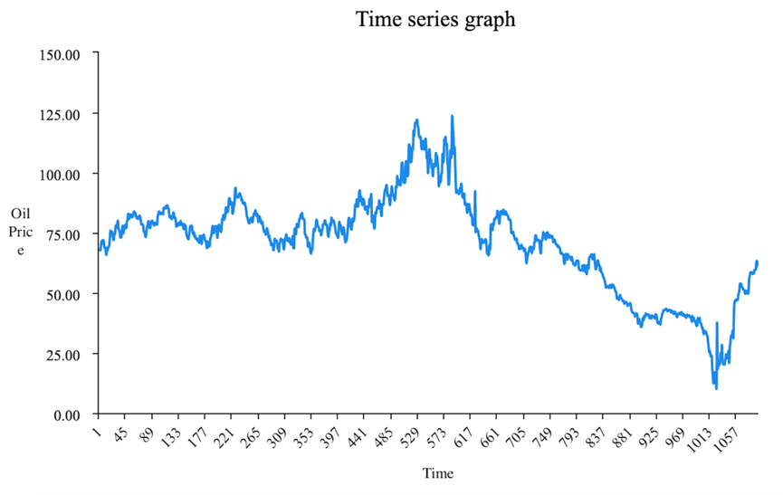
Figure 1: Time series graph of oil price

This research involves generating a dataset regarding global crude oil prices, alongside the need for further processing of several additional variables to ensure stationarity which is an important assumption for all kinds of time series modeling. The first ACF (Figure 2) of raw oil price series shows considerable autocorrelation with high data intensity, thereby suggesting that the time series was non-stationary. Stationarity was attained through first-order differencing. ACF and PACF plots for differenced data are shown in Figure 2 and 3, showing a clear decaying pattern and stationarity of differenced data. It was also augmented with an augmented Dickey-Fuller (ADF) test with statistic value -7.671 and p = 0.01 (Table 2) and thus rejected the null hypothesis of non-stationarity at a 1% significance level.

Table 2: Augmented dickey-fuller test results

Figure 2: ACF plots for differenced data

Figure 3: PACF plots for differenced data

3.2. Model selection and evaluation

The process of identification of the best ARIMA model had many possible combinations. Various configurations used optimization techniques with performance measured using Root Mean Square Error (RMSE) and Akaike Information Criterion (AIC). As listed in Table 3, the ARIMA(3,1,1) model attained the lowest AIC (2387.12) and a competitive RMSE (4.579), performing better than the others such as ARIMA(3,1,2) (AIC: 2389.04) and ARIMA(4,1,1) (AIC: 2396.18). The marginal variance in RMSE involved among the models stressed the preference of AIC to be parsimony in favor of ARIMA(3,1,1) regarding simplicity and accuracy. Therefore, using ARIMA(3,1,1) model is the best way to analyze and forecast the international oil price.

Table 3: ARIMA model performance comparison

3.3. Forecasting oil price dynamics

The ARIMA(3,1,1) model is selected to show the figure of real value in the past years and a prediction of the future trend.

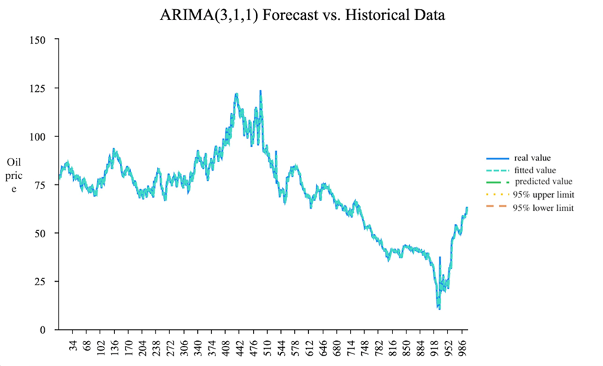
Figure 4: ARIMA(3,1,1) forecast vs. historical data

The selected ARIMA(3,1,1) model was used to make oil price forecasts over an entire year, from October 2023 to September 2024. The model shows, as shown in Figure 4 and Table 4, that there will be a short-lived price increase from 92.02 USD/barrel in October 2023 to gradually decline at 86.84 USD/barrel for September 2024. In line with the inherent volatility of oil markets, the increasing confidence intervals (e.g., 80% Confidence Interval (CI): 63.03-110.64; 95% CI: 50.43-123.25 for September 2024) indicate that there is a rising uncertainty across longer horizons.

Table 4: ARIMA(3,1,1) forecasts with confidence intervals

3.4. Residual diagnostics

The Q-Q plot is used to analyze the autocorrelation for the residuals and the distribution pattern.

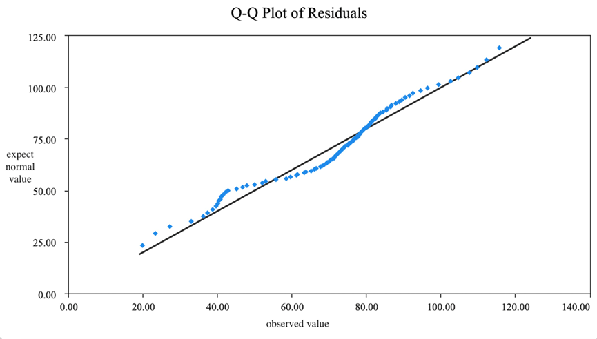
Figure 5: Q-Q plot of residuals

An analysis of the residuals was performed to verify model adequacy. There was no significant autocorrelation for the quantile-quantile (Q-Q) plot (Figure 5) indicated that they were approximately normally distributed with slight deviations in the tails. The Durbin-Watson statistic of 1.98 reflected no pronounced autocorrelation; besides the Ljung-Box test (p = 0.21) supported the null hypothesis of residual independence. The cumulative evidence confirmed the model's assumption that white noise residuals underpinned the development of the model.

3.5. Discussion

Performance on these tests confirms the robustness of the model. However, a discussion of the limitations is in order. The structural breaks in historical data which have been graphed in Figure 4. Since 2007, oil prices have likely experienced greater volatility due to geopolitical events, the 2008 financial crisis, and the shale oil boom. Constant parameters over time in an ARIMA framework mean that structural breaks of this nature make the model difficult to tune well. Extended short-run accuracy coupled with the bad idea of omitting long-run trends by excluding data through 2007 might improve model fit. In addition, external sources of economic disturbances: The incorporation of macroeconomic variables, such as GDP growth rates, interest rates, and indices of geopolitical risk into the model, has not been attempted, while they are known to be of episodic importance in influencing oil prices. The COVID-19 demand shock in 2020 or OPEC supply decisions would render such forecasts redundant. One possible avenue for use in improving adaptability is the hybridization of this with exogenous variables (ARIMAX) modeling or machine learning techniques. There are some reliefs in sight for energy-importing economies plagued by inflation, as oil prices are expected to fall to $87 a barrel by the end of 2024. Policymakers, however, need to be careful of upside risks such as supply disruptions or renewed demand out of emerging markets. Investors, meanwhile, can use the model confidence intervals to protect themselves against volatility in futures markets.

3.6. Comparative insights

The results coincide with prior studies which point towards dominant supply-demand fundamentals determining the long-run price of oil [10]. However, the model's inability to account for nonlinear interactions between financial speculation and geopolitical risk, a gap in recent literature, suggests that more advanced approaches should be possible [3, 6]. For illustration, Zhang et al. showed that using machine learning models for nonlinear inventory-price relationships increases forecasting accuracy, while Bastianin et al. warned against overfitting in complex models [5, 6].

4. Conclusion

This research has developed an ARIMA (3,1,1) model for crude oil price forecasting, providing useful outputs of Root Mean Squared Error (RMSE) of 4.579 and an Akaike Information Criterion (AIC) score of 2387.12. The model has demonstrated stability compared with classical statistical models, with a short-term volatility modeled to the moving average term (MA=1) and long-run trends modeled across the autoregressive term (AR=3). The selection of the ARIMA (3,1,1) model focuses on simplicity and accuracy, as demonstrated by both the RMSE and AIC statistics. These findings, aligning with historical studies, demonstrate the supply and demand fundamentals driving price, and reflect the challenges of modeling nonlinear market structures such as speculative bubbles or asymmetric responses to geopolitical shocks. Despite these useful outputs, limitations of this model are similar to substantial limitations in standard linear models. First, the model assumes stationarity and linear relationships (to account for temporal relationships in data) which may overlook or oversimplify the chaotic turbulent regime shifting nature of oil markets. For context, structural change, such as financial crisis in 2007-2008 or demand crash in 2020 due to COVID-19 pandemic, is beyond the model’s forecast. Second, the exclusion of exogenous variables in the model reduces usability in the rapidly changing market. Future research should be improved to address these limitations with introduction of hybrid models that use ARIMA and machine learning to capture nonlinear.

References

[1]. Hamilton, J.D. (1983) Oil and the Macroeconomy since World War II. Journal of Political Economy, 91(2), 228-248.
[2]. Kilian, L. (2009) Not All Oil Price Shocks Are Alike: Disentangling Demand and Supply Shocks in the Crude Oil Market. American Economic Review, 99(3), 1053-69.
[3]. Tang, K., et al. (2020) Speculation and Oil Price Dynamics. Energy Economics, 88, 104770.
[4]. Baumeister, C. and Peersman, G. (2013) Time-Varying Effects of Oil Supply Shocks on the US Economy. American Economic Journal, 5(4), 1-28.
[5]. Zhang, Y.J., et al. (2019) Forecasting Crude Oil Prices with Machine Learning. Energy, 188, 116062.
[6]. Bastianin, A., et al. (2021) Forecasting Oil Prices: A Review. Energy Economics, 99, 105283.
[7]. Wesseh, P.K. and Lin, B. (2020) Clean Energy Substitution and Oil Price Dynamics. Renewable Energy, 158, 420-429.
[8]. Kristjanpoller, W. and Hernández, L. (2017) Oil Price Forecasting Using Technical Indicators. Resources Policy, 52, 84-92
[9]. Lee, Y., et al. (2020) Structural Breaks in Oil Markets. Energy Economics, 86, 104634.
[10]. Narayan, P.K. (2019) Oil Price Drivers: A Meta-Analysis. Energy Policy, 131, 1-8.
Cite this article
Ge,R. (2025). The Research on Factors Influencing the Global Price of Crude Oil. Theoretical and Natural Science,105,8-14.
Data availability
The datasets used and/or analyzed during the current study will be available from the authors upon reasonable request.
Disclaimer/Publisher's Note
The statements, opinions and data contained in all publications are solely those of the individual author(s) and contributor(s) and not of EWA Publishing and/or the editor(s). EWA Publishing and/or the editor(s) disclaim responsibility for any injury to people or property resulting from any ideas, methods, instructions or products referred to in the content.
About volume
Volume title: Proceedings of the 3rd International Conference on Mathematical Physics and Computational Simulation
© 2024 by the author(s). Licensee EWA Publishing, Oxford, UK. This article is an open access article distributed under the terms and
conditions of the Creative Commons Attribution (CC BY) license. Authors who
publish this series agree to the following terms:
1. Authors retain copyright and grant the series right of first publication with the work simultaneously licensed under a Creative Commons
Attribution License that allows others to share the work with an acknowledgment of the work's authorship and initial publication in this
series.
2. Authors are able to enter into separate, additional contractual arrangements for the non-exclusive distribution of the series's published
version of the work (e.g., post it to an institutional repository or publish it in a book), with an acknowledgment of its initial
publication in this series.
3. Authors are permitted and encouraged to post their work online (e.g., in institutional repositories or on their website) prior to and
during the submission process, as it can lead to productive exchanges, as well as earlier and greater citation of published work (See
Open access policy for details).