1. Introduction

The nonlinear Schrödinger (NLS) equation

\( i{q_{t}}(x,t)={q_{xx}}(x,t)±2|q(x,t){|^{2}}q(x,t), \) (1)

which is an important model in nonlinear optics, providing good observation conditions for detecting PT symmetry theory [1-4]. The nonlinear Schrödinger (NLS) equation is widely applicable in physics, such as plasma physics [5-7], deep water waves [8-9], etc. Ablowitz and Musslimani proposed a non-local NLS equation, which is a new PT symmetric equation [10].

\( i{q_{t}}(x,t)={q_{xx}}(x,t)±2{q^{2}}(x,t){q^{*}}(-x,t), \) (2)

Equation (2) is Lax integrable, in fact, the AKNS system, under the new non-local symmetric reduction \( q(x,t)={q^{*}}(-x,t) \) , gives rise to Equation (2).

Ablowitz and Musslimani also studied the following integrable nonlocal discrete nonlinear Schrödinger equation [11].

\( i\frac{d{u_{n}}}{dt}={u_{n+1}}-2{u_{n}}+{u_{n-1}}±{u_{n}}u_{-n}^{*}({u_{n+1}}+{u_{n-1}}), \) (3)

where \( {u_{n}} \) is a time-dependent function of the integer \( n \) . Equation (3) has Lax pairs and infinite conservation law, therefore it is an integrable system. In reference [11], a discrete breathing soliton solution was obtained by establishing IST method of the decaying data. In [12], the N-soliton solution of integrable non-local discrete focused nonlinear non-linear Schrödinger (dNLS⁺) equation is constructed by bilinear method, and the asymptotic analysis of the double-soliton solution is given.

A generalization of the two-component discrete NLS [13], namely,

\( \begin{cases} \begin{array}{c} i{\dot{u}_{n}}+({u_{n+1}}+{u_{n-1}})(1+2{δ_{1}}{|{u_{n}}|^{2}}+2{δ_{2}}{|{v_{n}}|^{2}})-2{u_{n}}=0, \\ i{\dot{v}_{n}}+({v_{n+1}}+{v_{n-1}})(1+2{δ_{1}}{|{u_{n}}|^{2}}+2{δ_{2}}{|{v_{n}}|^{2}})-2{v_{n}}=0. \end{array} \end{cases} \) (4)

where the superscript ∗ means the complex conjugate, \( {δ_{j}}=±1,j=1,2 \) , Equation (4) holds significant mathematical and physical relevance. This system was first solved using the IST method in references [14][15]. More recently, a general multi-soliton solution expressed in terms of Pfaffians was derived in [16], where bright soliton solutions emerge in the focusing-focusing regime ( \( {δ_{1}}={δ_{2}}=1 \) ), while dark soliton solutions appear in the defocusing-defocusing case ( \( {δ_{1}}={δ_{2}}=-1 \) ). In [13], the Pfaffian form of the general bright dark soliton solution for the integrable semi discrete vector NLS equation was constructed using Hirota's bilinear method, and the bright-dark one-soliton solutions and two-soliton solutions of the two-component semi-discrete NLS equation were given. For Equation (4), with the reduction \( u_{n}^{*}(n,t)→u_{-n}^{*}(-n,t) \) , \( v_{n}^{*}(n,t)→v_{-n}^{*}(-n,t) \) , it can be obtained from the two-component non-local discrete NLS equation:

\( \begin{cases} \begin{array}{c} i{\dot{u}_{n}}+({u_{n+1}}+{u_{n-1}})(1+2{δ_{1}}{u_{n}}u_{-n}^{*}+2{δ_{2}}{v_{n}}v_{-n}^{*})-2{u_{n}}=0, \\ i{\dot{v}_{n}}+({v_{n+1}}+{v_{n-1}})(1+2{δ_{1}}{u_{n}}u_{-n}^{*}+2{δ_{2}}{v_{n}}v_{-n}^{*})-2{v_{n}}=0. \end{array} \end{cases} \) (5)

In this paper, we construct the bilinear form of the Equation (5) using the Hirota method, derive its soliton solutions, and present their dynamical behavior through numerical simulations.

2. The interaction of bright-bright soliton solutions

In this chapter, we seek bright-bright soliton solutions of the Equation (5) by bilinear methods. To derive the bilinear form, we perform dependent variable transformation on Equation (5):

\( {u_{n}}=\frac{{g_{n}}}{{f_{n}}},{v_{n}}=\frac{{h_{n}}}{{f_{n}}} \) (6)

where \( {g_{n}} \) , \( {h_{n}} \) , \( {f_{n}} \) are complex functions, the corresponding bilinear equations for Equation (5) is:

\( (i{D_{t}}+2(cosh{{D_{n}}}-1)){g_{n}}\cdot {f_{n}}=0, \) \( (i{D_{t}}+2(cosh{{D_{n}}}-1)){h_{n}}\cdot {f_{n}}=0, \) \( f_{-n}^{*}(cosh{{D_{n}}}-1){f_{n}}\cdot {f_{n}}=2{δ_{1}}{g_{n}}g_{-n}^{*}{f_{n}}+2{δ_{2}}{h_{n}}h_{-n}^{*}{f_{n}}. \) (7)

where D is the bilinear operator [17].

\( D_{t}^{l}D_{n}^{m}{f_{n}}(t)\cdot {g_{n}}(t)=(\frac{∂}{∂t}-\frac{∂}{∂t \prime }{)^{l}}(\frac{∂}{∂n}-\frac{∂}{∂n \prime }{)^{m}}{f_{n}}(t){g_{n \prime }}(t){|_{t=t \prime ,n=n \prime }}, \) \( exp{(}δ{D_{n}}){f_{n}}\cdot {g_{n}}={f_{n+δ}}{g_{n-δ}}. \) (8)

2.1. Bright-bright one-soliton solution

We will first focus on studying the one-soliton solutions of Equation (5). The following power series expansion is applied to \( {f_{n}} \) , \( {g_{n}} \) and \( {h_{n}} \) .

\( {f_{n}}=1+f_{n}^{(2)}{ε^{2}}+f_{n}^{(4)}{ε^{4}}+f_{n}^{(6)}{ε^{6}}+\cdot \cdot \cdot , \) \( {g_{n}}=g_{n}^{(1)}ε+g_{n}^{(3)}{ε^{3}}+g_{n}^{(5)}{ε^{5}}+\cdot \cdot \cdot , \) \( {h_{n}}=h_{n}^{(1)}ε+h_{n}^{(3)}{ε^{3}}+h_{n}^{(5)}{ε^{5}}+\cdot \cdot \cdot , \) (9)

in which ε denotes a sufficiently small parameter. we cut off expression (9) to \( {f_{n}}=1+f_{n}^{(2)}{ε^{2}} \) , \( {g_{n}}=g_{n}^{(1)}ε \) , \( {h_{n}}=h_{n}^{(1)}ε \) , these expressions are then substituted into the bilinear formulation (7). By comparing terms order by order in powers of ε, we obtain the following system of equations:

\( {A_{1}}g_{n}^{(1)}\cdot 1=0，{A_{1}}h_{n}^{(1)}\cdot 1=0， \) (10)

\( {A_{2}}(1\cdot f_{n}^{(2)}+f_{n}^{(2)}\cdot 1)=2{δ_{1}}g_{n}^{(1)}g_{-n}^{(1)*}+2{δ_{2}}h_{n}^{(1)}h_{-n}^{(1)*}， \) (11)

\( {A_{1}}g_{n}^{(1)}f_{n}^{(2)}=0,{A_{1}}h_{n}^{(1)}f_{n}^{(2)}=0, \) (12)

\( {A_{2}}f_{n}^{(2)}\cdot f_{n}^{(2)}+f_{-n}^{(2)*}{A_{2}}(1\cdot f_{n}^{(2)}+f_{n}^{(2)}\cdot 1)=2{δ_{1}}g_{n}^{(1)}g_{-n}^{(1)*}f_{n}^{(2)}+2{δ_{2}}h_{n}^{(1)}h_{-n}^{(1)*}f_{n}^{(2)}， \) (13)

\( f_{-n}^{(2)*}{A_{2}}f_{n}^{(2)}\cdot f_{n}^{(2)}=0, \) (14)

where the bilinear operators \( {A_{1}} \) and \( {A_{2}} \) are given by

\( {A_{1}}=i{D_{t}}+2(cosh{{D_{n}}}-1) \) \( {A_{2}}=cosh{{D_{n}}}-1 \) (15)

Assuming \( g_{n}^{(1)}=α{e^{ξ}} \) , \( h_{n}^{(1)}=β{e^{ξ}} \) , \( f_{n}^{(2)}=θ{e^{ξ+ξ_{-n}^{*}}} \) with \( ξ=κn+ωt \) , \( ξ_{-n}^{*}=-{κ^{*}}n+{ω^{*}}t \) , and \( α \) , \( β \) are any complex parameters. Equation (10) and (11) yield the dispersion relation \( ω=2i(coshκ-1) \) and the value of \( θ=\frac{{δ_{1}}{|α|^{2}} +{δ_{2}}{|β|^{2}}}{2}{sinh^{-2}}\frac{κ-{κ^{*}}}{2} \) . Besides, the remaining equations are inherently fulfilled without additional constraints, the one-soliton solution for Equation (5) can be expressed in the following form:

\( \begin{cases}\begin{matrix}{u_{n}}=\frac{εα{e^{κn+ωt}}}{1+{ε^{2}}θ{e^{(κ-κ*)n+(ω+ω*)t}}} \\ {v_{n}}=\frac{εβ{e^{κn+ωt}}}{1+{ε^{2}}θ{e^{(κ-κ*)n+(ω+ω*)t}}} \\ \end{matrix}\end{cases} \) (16)

Setting \( κ=a+ib(b≠0) \) , Equation (16) becomes

\( \begin{cases}\begin{matrix}{u_{n}}=\frac{εα{e^{an-2tsinh{a}sin{b}}}{e^{i(bn+2t(cosh{a}cos{b}-1))}}}{1-{ε^{2}}\frac{({δ_{1}}{|α|^{2}}+{δ_{2}}{|β|^{2}}){csc^{2}}{b}}{2}{e^{2ibn-4tsinh{a}sin{b}}}} \\ {v_{n}}=\frac{εβ{e^{an-2tsinh{a}sin{b}}}{e^{i(bn+2t(cosh{a}cos{b}-1))}}}{1-{ε^{2}}\frac{({δ_{1}}{|α|^{2}}+{δ_{2}}{|β|^{2}}){csc^{2}}{b}}{2}{e^{2ibn-4tsinh{a}sin{b}}}} \\ \end{matrix}\end{cases} \) (17)

Setting \( ε=1 \) , Equation (16) can be written as

\( \begin{cases}\begin{matrix}{u_{n}}=\frac{α}{\sqrt[]{2({δ_{1}}{|α|^{2}}+{δ_{2}}{|β|^{2}})}}{e^{\frac{κ+κ*}{2}n+\frac{ω-ω*}{2}t}}sech{(}\frac{κ-κ*}{2}n+\frac{ω+ω*}{2}t-ϕ)sinh{(}\frac{κ-κ*}{2}), \\ {v_{n}}=\frac{β}{\sqrt[]{2({δ_{1}}{|α|^{2}}+{δ_{2}}{|β|^{2}})}}{e^{\frac{κ+κ*}{2}n+\frac{ω-ω*}{2}t}}sech{(}\frac{κ-κ*}{2}n+\frac{ω+ω*}{2}t-ϕ)sinh{(}\frac{κ-κ*}{2}). \\ \end{matrix}\end{cases} \) (18)

in which \( ϕ=ln(\sqrt[]{\frac{2}{{δ_{1}}{|α|^{2}} +{δ_{2}}{|β|^{2}}}}sinh\frac{|κ-{κ^{*}}|}{2}) \) . As \( a≠0 \) , and \( b≠lπ \) , \( l∈Z \) , the singular point of one-soliton occurs at \( (n, t)=(\frac{kπ}{b}, \frac{-4}{sinha sinb}ln\frac{2{sin^{2}}b}{{ε^{2}}({δ_{1}}{|α|^{2}} +{δ_{2}}{|β|^{2}})} \) ), \( k∈Z \) . When \( ε=1 \) and \( κ=a+ib,(b≠0) \) , we can get:

\( \begin{cases}\begin{matrix}|{u_{n}}|=\frac{2|α|{e^{an-2tsinh{a}sin{b}}}}{\sqrt[]{4-4{e^{-4tsin{b}sinh{a}}}cos{(}2bn){csc^{2}}{b}({δ_{1}}{|α|^{2}}+{δ_{2}}{|β|^{2}})+{e^{-8tsin{b}sinh{a}}}{csc^{4}}{b}({δ_{1}}{|α|^{2}}+{δ_{2}}{|β|^{2}}{)^{2}}}}, \\ |{v_{n}}|=\frac{2|β|{e^{an-2tsinh{a}sin{b}}}}{\sqrt[]{4-4{e^{-4tsin{b}sinh{a}}}cos{(}2bn){csc^{2}}{b}({δ_{1}}{|α|^{2}}+{δ_{2}}{|β|^{2}})+{e^{-8tsin{b}sinh{a}}}{csc^{4}}{b}({δ_{1}}{|α|^{2}}+{δ_{2}}{|β|^{2}}{)^{2}}}}. \\ \end{matrix}\end{cases} \) (19)

Specifically, when \( a=0 \) , Equation (19) can be expressed in the following form:

\( \begin{cases}\begin{matrix}|{u_{n}}|=\frac{2|α|}{\sqrt[]{4-4cos{(}2bn){csc^{2}}{b}({δ_{1}}{|α|^{2}}+{δ_{2}}{|β|^{2}})+{csc^{4}}{b}{({δ_{1}}{|α|^{2}}+{δ_{2}}{|β|^{2}})^{2}}}}, \\ |{v_{n}}|=\frac{2|β|}{\sqrt[]{4-4cos{(}2bn){csc^{2}}{b}({δ_{1}}{|α|^{2}}+{δ_{2}}{|β|^{2}})+{csc^{4}}{b}{({δ_{1}}{|α|^{2}}+{δ_{2}}{|β|^{2}})^{2}}}}. \\ \end{matrix}\end{cases} \) (20)

with the period \( M=\frac{π}{b} \) . Using Mathematica software, the soliton diagrams are given as follows. In Figure 1, using parameter \( κ=0.3i,{ δ_{1}}={δ_{2}}=1, α=1, β=0.7, \) we can obtain that one-soliton solutions are periodic solutions. In Figure 2, using parameter \( κ=0.2+0.8i, { δ_{1}}={δ_{2}}=1, α=-1+0.5i \) , and \( β=-0.1-0.2i \) , we can obtain the one-soliton solutions are singular solutions.

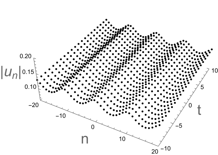
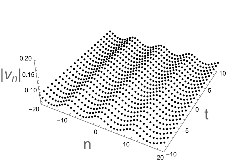
Figure 1: Period solutions \( {u_{n}} \) and \( {v_{n}} \) with parameter as: \( κ=0.3i,{δ_{1}}={δ_{2}}=1, α=1, β=0.7 \) .

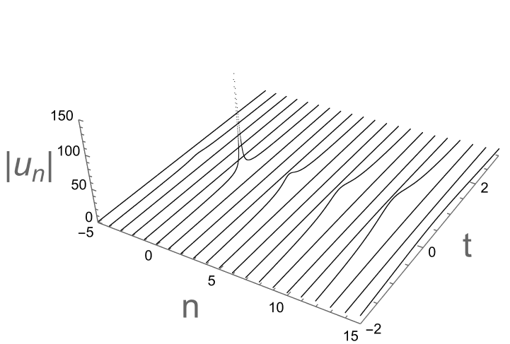
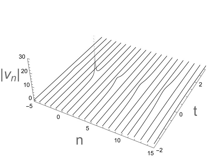
Figure 2: Singular solutions with parameters as:

\( κ=0.2+0.8i, {δ_{1}}={δ_{2}}=1, α=-1+0.5i,β=-0.1-0.2i \)

We proceed to examine the continuum limit approximation of the discrete one-soliton solution (16). Set \( {u_{n}}(t)=εu(x, τ) \) , \( x=nε \) , \( τ={ε^{2}}t \) , and \( κ=λε \) , when \( ε→0 \) , the one-soliton solution (16) converges to

\( \begin{cases}\begin{matrix}u(x,τ)=\frac{α{e^{λx+i{λ^{2}}τ}}}{1+\frac{2({δ_{1}}{|α|^{2}}+{δ_{2}}{|β|^{2}})}{{(λ-λ*)^{2}}}{e^{(λ-λ*)x+i({λ^{2}}-λ{*^{2}})τ}}}, \\ v(x,τ)=\frac{β{e^{λx+i{λ^{2}}τ}}}{1+\frac{2({δ_{1}}{|α|^{2}}+{δ_{2}}{|β|^{2}})}{{(λ-λ*)^{2}}}{e^{(λ-λ*)x+i({λ^{2}}-λ{*^{2}})τ}}}. \\ \end{matrix}\end{cases} \) (21)

This represents a novel soliton solution to the integrable coupled discrete nonlocal nonlinear Schrödinger equation. Set \( λ={μ_{1}}+i{μ_{2}} \) , then:

\( \begin{cases}\begin{matrix}u(x,τ)=\frac{α{e^{i({μ_{2}}x+({{μ_{1}}^{2}}-{{μ_{2}}^{2}})τ)}}{e^{{μ_{1}}x-2{μ_{1}}{μ_{2}}τ}}}{1-\frac{{δ_{1}}{|α|^{2}}+{δ_{2}}{|β|^{2}}}{2{{μ_{2}}^{2}}}{e^{2i{μ_{2}}x-4{μ_{1}}{μ_{2}}τ}}}, \\ v(x,τ)=\frac{β{e^{i({μ_{2}}x+({{μ_{1}}^{2}}-{{μ_{2}}^{2}})τ)}}{e^{{μ_{1}}x-2{μ_{1}}{μ_{2}}τ}}}{1-\frac{{δ_{1}}{|α|^{2}}+{δ_{2}}{|β|^{2}}}{2{{μ_{2}}^{2}}}{e^{2i{μ_{2}}x-4{μ_{1}}{μ_{2}}τ}}}. \\ \end{matrix}\end{cases} \) (22)

The singularity of this solution appears at \( (x,τ)=(\frac{kπ}{{μ_{2}}},\frac{ln⁡(4{{μ_{2}}^{2}})}{4{μ_{1}}{μ_{2}}}),k∈Z \) . The solution (22) does not exhibit breather characteristics in either the temporal or spatial domain.

2.2. Bright-bright two-soliton solution

It should be emphasized that multiple solutions exist for Equation (5). For deriving the coupled bright-bright two-soliton solution, we solve Equation (5) as

\( {g_{n}}=g_{n}^{(1)}ε+g_{n}^{(3)}{ε^{3}}, {h_{n}}=h_{n}^{(1)}ε+h_{n}^{(3)}{ε^{3}}, {f_{n}}=1+f_{n}^{(2)}{ε^{2}}+f_{n}^{(4)}{ε^{4}}. \) (23)

We obtain a series of bilinear equations

\( {A_{1}}g_{n}^{(1)}\cdot 1=0，{A_{1}}h_{n}^{(1)}\cdot 1=0， \) \( {A_{2}}(1\cdot f_{n}^{(2)}+f_{n}^{(2)}\cdot 1)=2{δ_{1}}g_{n}^{(1)}g_{-n}^{(1)*}+2{δ_{2}}h_{n}^{(1)}h_{-n}^{(1)*}， \) \( {A_{1}}(g_{n}^{(1)}\cdot f_{n}^{(2)}+g_{n}^{(3)}\cdot 1=0，{A_{1}}(h_{n}^{(1)}\cdot f_{n}^{(2)}+h_{n}^{(3)}\cdot 1)=0， \) \( {A_{2}}(1\cdot f_{n}^{(4)}+f_{n}^{(2)}\cdot f_{n}^{(2)}+f_{n}^{(4)}\cdot 1)+f_{-n}^{(2)*}{A_{2}}(1\cdot f_{n}^{(2)}+f_{n}^{(2)}\cdot 1) \) \( =2{δ_{1}}(g_{n}^{(1)}g_{-n}^{(1)*}f_{n}^{(2)}+g_{n}^{(3)}g_{-n}^{(1)*}+g_{n}^{(1)}g_{-n}^{(3)*})+2{δ_{2}}(h_{n}^{(1)}h_{-n}^{(1)*}f_{n}^{(2)}+h_{n}^{(3)}h_{-n}^{(1)*}+h_{n}^{(1)}h_{-n}^{(3)*}), \) \( {A_{2}}(f_{n}^{(2)}\cdot f_{n}^{(4)}+f_{n}^{(4)}\cdot f_{n}^{(2)}+f_{-n}^{(2)*}{A_{2}}(1\cdot f_{n}^{(4)}+f_{n}^{(2)}\cdot f_{n}^{(2)}+f_{n}^{(4)}\cdot 1)+f_{-n}^{(4)*}{A_{2}}(1\cdot f_{n}^{(2)}+f_{n}^{(2)}\cdot 1) \) \( =2{δ_{1}}(g_{n}^{(1)}g_{-n}^{(1)*}f_{n}^{(4)}+g_{n}^{(3)}g_{-n}^{(1)*}f_{n}^{(2)}+g_{n}^{(1)}g_{-n}^{(3)*}f_{n}^{(2)}+g_{n}^{(3)}g_{-n}^{(3)*}) \) \( +2{δ_{2}}(h_{n}^{(1)}h_{-n}^{(1)*}f_{n}^{(4)}+h_{n}^{(3)}h_{-n}^{(1)*}f_{n}^{(2)}+h_{n}^{(1)}h_{-n}^{(3)*}f_{n}^{(2)}+h_{n}^{(3)}h_{-n}^{(3)*}), \) \( {A_{1}}g_{n}^{(3)}\cdot f_{n}^{(4)}=0,{A_{1}}h_{n}^{(3)}\cdot f_{n}^{(4)}=0, \) \( {A_{2}}f_{n}^{(4)}\cdot f_{n}^{(4)}+f_{-n}^{(2)*}{A_{2}}(f_{n}^{(2)}\cdot f_{n}^{(4)}+f_{n}^{(4)}\cdot f_{n}^{(2)})+f_{-n}^{(4)*}{A_{2}}(1\cdot f_{n}^{(4)}+f_{n}^{(2)}\cdot f_{n}^{(2)}+f_{n}^{(4)}\cdot 1) \) \( =2{δ_{1}}(g_{n}^{(3)}g_{-n}^{(1)*}f_{n}^{(4)}+g_{n}^{(1)}g_{-n}^{(3)*}f_{n}^{(4)}+g_{n}^{(3)}g_{-n}^{(3)*}f_{n}^{(2)}) \) \( +2{δ_{2}}(h_{n}^{(3)}h_{-n}^{(1)*}f_{n}^{(4)}+h_{n}^{(1)}h_{-n}^{(3)*}f_{n}^{(4)}+h_{n}^{(3)}h_{-n}^{(3)*}f_{n}^{(2)}), \) \( f_{-n}^{(2)*}{A_{2}}f_{n}^{(4)}\cdot f_{n}^{(4)}+f_{-n}^{(4)*}{A_{2}}(f_{n}^{(2)}\cdot f_{n}^{(4)}+f_{n}^{(4)}\cdot f_{n}^{(2)})=2{δ_{1}}g_{n}^{(3)}g_{-n}^{(3)*}f_{n}^{(4)}+2{δ_{2}}h_{n}^{(3)}h_{-n}^{(3)*}f_{n}^{(4)}, \) \( f_{n}^{(4)*}{A_{2}}f_{n}^{(4)}\cdot f_{n}^{(4)}=0. \) (24)

to solve these equations, we let

\( g_{n}^{(1)}={α_{1}}{e^{{ξ_{1}}}}+{α_{2}}{e^{{ξ_{2}}}},g_{n}^{(3)}={a_{1,2,1*}}{e^{{ξ_{1}}+{ξ_{2}}+ξ_{1,-n}^{*}}}+{a_{1,2,2*}}{e^{{ξ_{1}}+{ξ_{2}}+ξ_{2,-n}^{*}}}, \) \( h_{n}^{(1)}={β_{1}}{e^{{ξ_{1}}}}+{β_{2}}{e^{{ξ_{2}}}},h_{n}^{(3)}={b_{1,2,1*}}{e^{{ξ_{1}}+{ξ_{2}}+ξ_{1,-n}^{*}}}+{b_{1,2,2*}}{e^{{ξ_{1}}+{ξ_{2}}+ξ_{2,-n}^{*}}}, \) \( f_{n}^{(2)}={a_{1,1*}}{e^{{ξ_{1}}+ξ_{1,-n}^{*}}}+{a_{1,2*}}{e^{{ξ_{1}}+ξ_{2,-n}^{*}}}+{a_{2,1*}}{e^{{ξ_{2}}+ξ_{1,-n}^{*}}}+{a_{2,2*}}{e^{{ξ_{2}}+ξ_{2,-n}^{*}}}, \) \( f_{n}^{(4)}={a_{1,2,1*,2*}}{e^{{ξ_{1}}+{ξ_{2}}+ξ_{1,-n}^{*}+ξ_{2,-n}^{*}}}. \) (25)

and for \( j=1,2 \)

\( {ξ_{j}}={κ_{j}}n+{ω_{j}}t+ξ_{j}^{0}, ξ_{j,-n}^{*}=-κ_{j}^{*}n+ω_{j}^{*}t+ξ_{j}^{0*}. \) (26)

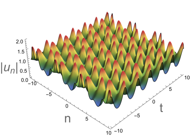
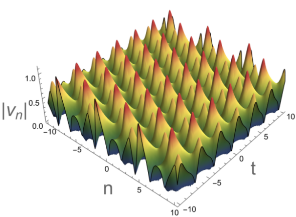
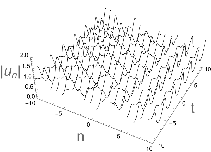
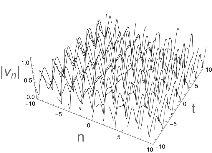
Figure 3: Double spatial period solutions with \( {κ_{1}}=-2i,{κ_{2}}=i \) .

we can obtain the dispersion relation \( {ω_{j}}=2i(cosh{κ_{j}}-1) \) . Some important coefficients of the soliton solutions are obtained through complex calculations as following

\( {a_{l,m*}}=\frac{{α_{l}}α_{m}^{*}+{β_{l}}β_{m}^{*}}{2}{sinh^{-2}}{\frac{{κ_{l}}-κ_{m}^{*}}{2}}, \) \( {a_{1,2,1*}}=\frac{1}{{p_{12}}}({α_{1}}{a_{2,1*}}{p_{1,1*}}-{α_{2}}{a_{1,1*}}{p_{2,1*}}),{a_{1,2,2*}}=\frac{1}{{p_{12}}}({α_{1}}{a_{2,2*}}{p_{1,2*}}-{α_{2}}{a_{1,2*}}{p_{2,2*}}), \) \( {b_{1,2,1*}}=\frac{1}{{p_{12}}}({β_{1}}{a_{2,1*}}{p_{1,1*}}-{β_{2}}{a_{1,1*}}{p_{2,1*}}),{b_{1,2,2*}}=\frac{1}{{p_{12}}}({β_{1}}{a_{2,2*}}{p_{1,2*}}-{β_{2}}{a_{1,2*}}{p_{2,2*}}), \) \( {a_{1,2,1*,2*}}=-4({|{α_{1}}|^{2}}+{|{β_{1}}|^{2}})({|{α_{2}}|^{2}}+{|{β_{2}}|^{2}})\frac{{p_{12*}}{p_{21*}}}{{p_{12}}{p_{1*2*}}}\frac{{e^{2{κ_{1R}}+2{κ_{2R}}}}}{{({e^{{κ_{1}}}}-{e^{κ_{1}^{*}}})^{2}}{({e^{{κ_{2}}}}-{e^{κ_{2}^{*}}})^{2}}} \) \( +4({α_{1}}α_{2}^{*}+{β_{1}}β_{2}^{*})({α_{2}}α_{1}^{*}+{β_{2}}β_{1}^{*})\frac{{p_{11*}}{p_{22*}}}{{p_{12}}{p_{1*2*}}}\frac{{e^{2{κ_{1R}}+2{κ_{2R}}}}}{{({e^{{κ_{2}}}}-{e^{κ_{1}^{*}}})^{2}}{({e^{{κ_{1}}}}-{e^{κ_{2}^{*}}})^{2}}}. \) (27)

where

\( {p_{12}}=\frac{1+{e^{{κ_{1}}+{κ_{2}}}}}{{e^{{κ_{1}}}}-{e^{{κ_{2}}}}},{p_{1*2*}}=\frac{1+{e^{κ_{1}^{*}+κ_{2}^{*}}}}{{e^{κ_{1}^{*}}}-{e^{κ_{2}^{*}}}},{p_{ij*}}=\frac{1+{e^{{κ_{i}}+κ_{j}^{*}}}}{{e^{{κ_{i}}}}-{e^{κ_{j}^{*}}}}, \) (28)

Therefore, for \( ε=1 \) the two-soliton solution is

\( \begin{cases}\begin{matrix}{u_{n}}=\frac{{α_{1}}{e^{{ξ_{1}}}}+{α_{2}}{e^{{ξ_{2}}}}+{a_{1,2,1*}}{e^{{ξ_{1}}+{ξ_{2}}+ξ_{1,-n}^{*}}}+{a_{1,2,2*}}{e^{{ξ_{1}}+{ξ_{2}}+ξ_{2,-n}^{*}}}}{1+{a_{1,1*}}{e^{{ξ_{1}}+ξ_{1,-n}^{*}}}+{a_{1,2*}}{e^{{ξ_{1}}+ξ_{2,-n}^{*}}}+{a_{2,1*}}{e^{{ξ_{2}}+ξ_{1,-n}^{*}}}+{a_{2,2*}}{e^{{ξ_{2}}+ξ_{2,-n}^{*}}}+{a_{1,2,1*,2*}}{e^{{ξ_{1}}+{ξ_{2}}+ξ_{1,-n}^{*}+ξ_{2,-n}^{*}}}} \\ {v_{n}}=\frac{{β_{1}}{e^{{ξ_{1}}}}+{β_{2}}{e^{{ξ_{2}}}}+{b_{1,2,1*}}{e^{{ξ_{1}}+{ξ_{2}}+ξ_{1,-n}^{*}}}+{b_{1,2,2*}}{e^{{ξ_{1}}+{ξ_{2}}+ξ_{2,-n}^{*}}}}{1+{a_{1,1*}}{e^{{ξ_{1}}+ξ_{1,-n}^{*}}}+{a_{1,2*}}{e^{{ξ_{1}}+ξ_{2,-n}^{*}}}+{a_{2,1*}}{e^{{ξ_{2}}+ξ_{1,-n}^{*}}}+{a_{2,2*}}{e^{{ξ_{2}}+ξ_{2,-n}^{*}}}+{a_{1,2,1*,2*}}{e^{{ξ_{1}}+{ξ_{2}}+ξ_{1,-n}^{*}+ξ_{2,-n}^{*}}}} \\ \end{matrix}\end{cases} \) (29)

the solution \( {u_{n}},{v_{n}} \) are double spatial period solutions. In Figure 3, discrete and corresponding continuous double spatial period soliton diagrams are plotted under specific parameters.

3. The interaction of dark-dark soliton solutions

This section focuses on the exploration of coupled dark-dark soliton solutions of the Equation (5). By using the dependent variable transformations

\( {u_{n}}={ρ_{1}}(i{k_{1}}{)^{n}}\frac{{g_{n}}}{{f_{n}}}{e^{({ω_{1}}-2i)t}},{v_{n}}={ρ_{2}}(i{k_{2}}{)^{n}}\frac{{h_{n}}}{{f_{n}}}{e^{({ω_{2}}-2i)t}}. \) (30)

where \( {f_{n}} \) is a real function and \( { g_{n}},{ h_{n}} \) are complex functions, \( {ω_{j}}=m(k_{j}^{-1}-{k_{j}}) \) , \( {k_{j}} \) are complex constants with \( {k_{j}}=-k_{j}^{*},j=1,2 \) , Equation (5) can be expressed in the following bilinear form:

\( ({ω_{1}}+{D_{t}}){g_{n}}\cdot {f_{n}}+m({k_{1}}{g_{n+1}}{f_{n-1}}-k_{1}^{-1}{g_{n-1}}{f_{n+1}})=0, \) \( ({ω_{2}}+{D_{t}}){h_{n}}\cdot {f_{n}}+m({k_{2}}{h_{n+1}}{f_{n-1}}-k_{2}^{-1}{h_{n-1}}{f_{n+1}})=0, \) \( f_{-n}^{*}(m{f_{n+1}}{f_{n-1}}-f_{n}^{2})=2{δ_{1}}{|{ρ_{1}}|^{2}}{g_{n}}g_{-n}^{*}{f_{n}}+2{δ_{2}}{|{ρ_{2}}|^{2}}{h_{n}}h_{-n}^{*}{f_{n}}. \) (31)

Expand \( {f_{n}},{ g_{n}} \) and \( {h_{n}} \) in Equation (31) as follows:

\( {f_{n}}=1+f_{n}^{(2)}{ε^{2}}+f_{n}^{(4)}{ε^{4}}+f_{n}^{(6)}{ε^{6}}+\cdot \cdot \cdot , \) \( {g_{n}}=1+g_{n}^{(2)}{ε^{2}}+g_{n}^{(4)}{ε^{4}}+g_{n}^{(6)}{ε^{6}}+\cdot \cdot \cdot , \) \( {h_{n}}=1+h_{n}^{(2)}{ε^{2}}+h_{n}^{(4)}{ε^{4}}+h_{n}^{(6)}{ε^{6}}+\cdot \cdot \cdot . \) (32)

for obtaining the two dark-dark solution, functions are assumed to be

\( {f_{n}}=1+f_{n}^{(2)}{ε^{2}}+f_{n}^{(4)}{ε^{4}},{g_{n}}=1+g_{n}^{(2)}{ε^{2}}+g_{n}^{(4)}{ε^{4}},{h_{n}}=1+h_{n}^{(2)}{ε^{2}}+h_{n}^{(4)}{ε^{4}}. \) (33)

Substituting Equation (32) into Equation (31), the forms of \( {g_{n}} \) , \( {h_{n}} \) , \( {f_{n}} \) are assumed to be

\( g_{n}^{(2)}={a_{1}}{e^{{ξ_{1}}}}+{a_{2}}{e^{{ξ_{1,-n}}}},h_{n}^{(2)}={b_{1}}{e^{{ξ_{1}}}}+{b_{2}}{e^{{ξ_{1,-n}}}},f_{n}^{(2)}={e^{{ξ_{1}}}}+{e^{{ξ_{1,-n}}}}, \) \( g_{n}^{(4)}={a_{1}}{a_{2}}M{e^{{ξ_{1}}+{ξ_{1,-n}}}},h_{n}^{(4)}={b_{1}}{b_{2}}M{e^{{ξ_{1}}+{ξ_{1,-n}}}},f_{n}^{(4)}=M{e^{{ξ_{1}}+{ξ_{1,-n}}}}. \) (34)

where \( {ξ_{1}}=Pn+Ωt+ξ_{1}^{0} \) , \( {ξ_{1,-n}}=-Pn+Ωt+ξ_{1}^{0} \) , \( m=1+2{δ_{1}}{|{ρ_{1}}|^{2}}+2{δ_{2}}{|{ρ_{2}}|^{2}} \) , \( {ω_{j}}+m({k_{j}}-k_{j}^{-1})=0 \) , and \( P \) , \( Ω \) , \( ξ_{1}^{0} \) are real constants, \( {a_{1}},{a_{2}},{b_{1}},{b_{2}} \) are arbitrary complex constants, when \( {k_{1}}={k_{2}}=-i \) , then \( {ω_{1}}={ω_{2}}=2mi \) , \( Ω \) and \( P \) satisfy the following equation

\( m{e^{-3P}}({e^{P}}-1{)^{2}}({Ω^{2}}{e^{2P}}+m({e^{P}}-1{)^{2}}(2{e^{P}}(m-2)+m+m{e^{2P}}))=0. \) (35)

We get the two dark-dark solution for Equation (5) as

\( \begin{cases}\begin{matrix}{u_{n}}={ρ_{1}}(i{k_{1}}{)^{n}}{e^{({ω_{1}}-2i)t}}\frac{1+{a_{1}}{e^{{ξ_{1}}}}+{a_{2}}{e^{{ξ_{1,-n}}}}+{a_{1}}{a_{2}}M{e^{{ξ_{1}}+{ξ_{1,-n}}}}}{1+{e^{{ξ_{1}}}}+{e^{{ξ_{1,-n}}}}+M{e^{{ξ_{1}}+{ξ_{1,-n}}}}}, \\ {v_{n}}={ρ_{2}}(i{k_{2}}{)^{n}}{e^{({ω_{2}}-2i)t}}\frac{1+{b_{1}}{e^{{ξ_{1}}}}+{b_{2}}{e^{{ξ_{1,-n}}}}+{b_{1}}{b_{2}}M{e^{{ξ_{1}}+{ξ_{1,-n}}}}}{1+{e^{{ξ_{1}}}}+{e^{{ξ_{1,-n}}}}+M{e^{{ξ_{1}}+{ξ_{1,-n}}}}}. \\ \end{matrix}\end{cases} \) (36)

where

\( {a_{1}}={a_{2}}={b_{1}}={b_{2}}=\frac{Ω+im({e^{P}}+{e^{-P}}-2)}{Ω-im({e^{P}}+{e^{-P}}-2)}, \) \( M=\frac{{e^{-3P}}(1+{e^{P}}{)^{2}}({m^{2}}({e^{P}}-1{)^{4}}+{e^{2P}}{Ω^{2}})}{4{Ω^{2}}}. \) (37)

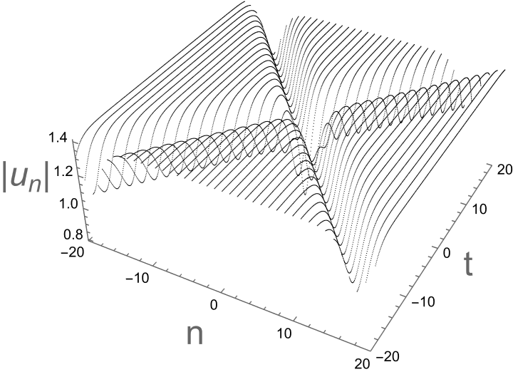
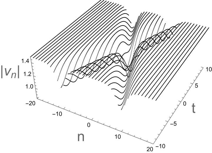
Figure 4: dark-dark soliton solutions with parameters as:

\( {k_{1}}={k_{2}}=-i,P=-1,{δ_{1}}=1,{δ_{2}}=-1,{ρ_{1}}=1-i,{ρ_{2}}=1+1.1i \) .

Formally speaking, the expansion of \( {f_{n}} \) , \( { g_{n}} \) and \( {h_{n}} \) in this section and the form of solutions are derived from continuous equations, However, in continuous systems, they correspond to breathers, while in non-local systems, they exhibit dark-dark soliton waves, dark-antidark soliton waves or antidark-antidark soliton waves. In Figure 4, we obtain the dark-dark soliton waves with the parameters: \( {k_{1}}={k_{2}}=-i,P=-1,{δ_{1}}=1,{δ_{2}}=-1,{ρ_{1}}=1-i,{ρ_{2}}=1+1.1i \) .

4. Conclusion

The coupled discrete non-local nonlinear Schrödinger Equation (5) represents a novel integrable system in discrete mathematics. This study employs the Hirota bilinear approach to derive the bilinear representation of this coupled nonlocal discrete system. Through systematic analysis, we establish both bright-bright single and two-soliton solutions, followed by the development of bilinear expansions for dark-dark soliton configurations. Furthermore, computational methods are implemented to generate graphical representations of these soliton solutions. We found that compared to non-local NLS equations, integrable coupled discrete non-local NLS equations have a richer variety of soliton solution types, and the interactions between soliton solutions and the evolution properties of solutions over time are also significantly different.

References

[1]. Rüter C.E., Makris K.G., El-Ganainy R., Christodoulides D.N., Segev M., Kip D., Observation of parity-time symmetry in optics, Nat. Phys., 2010, 6, 192-195.
[2]. Regensburger A., Bersch C., Miri M.A., Onishchukov G., Christodoulides D.N., Peschel U., Parity-time synthetic photonic lattices, Nature, 2012, 488, 167-171.
[3]. Regensburger A., Miri M.A., Bersch C., Nager J., Onishchukov G., Christodoulides D.N., Peschel U., Observation of defect states in PT-symmetric optical lattices, Phys. Rev. Lett., 2013, 110, 223902.
[4]. Guo A., Salamo G.J., Duchesne D., Morandotti R., Volatier-Ravat M., Aimez V., Siviloglou G.A., Christodoulides D.N., Observation of PT-symmetry breaking in complex optical potentials, Phys. Rev. Lett., 2009, 103, 093902.
[5]. Zakharov V.E., Collapse of Langmuir waves, Sov. Phys. JETP, 1972, 35, 908-914.
[6]. Zakharov V., Shabat A., Exact theory of two-dimensional self-focusing and one-dimensional self-modulation of waves in nonlinear media, Sov. Phys. JETP, 1972, 34, 62-69.
[7]. Zakharov V., Shabat A., Interaction between solitons in a stable medium, Sov. Phys. JETP, 1973, 37, 823-828.
[8]. Benney D.J., Newell A.C., The propagation of nonlinear wave envelopes, Stud. Appl. Math., 1967, 46, 133-139.
[9]. Zvezdin A.K., Popkov A.F., Contribution to the nonlinear theory of magnetostatic spin waves, Sov. Phys. JETP, 1983, 57, 350-355.
[10]. M.J. Ablowitz, Z.H. Musslimani, Integrable nonlocal nonlinear Schrödinger equation, Phys. Rev. Lett. 110 (2013) 064105.
[11]. Ablowitz M.J., Musslimani Z.H., Integrable discrete PT symmetric model, Phys. Rev. E, 2014, 90, 032912.
[12]. Ma L.Y., Zhu Z.N., N-soliton solution for an integrable nonlocal discrete focusing nonlinear Schrödinger equation, Appl. Math. Lett., 2016, 59, 115-121.
[13]. Ma L.Y., Zhu Z.N., N-soliton solution for an integrable nonlocal discrete focusing nonlinear Schrödinger equation, Appl. Math. Lett., 2016, 59, 115-121.
[14]. Tsuchida T., Integrable discretization of coupled nonlinear Schrödinger equations, Rep. Math. Phys., 2000, 46, 269-278.
[15]. Tsuchida T., Ujino H., Wadati M., Integrable semi-discretization of the coupled nonlinear Schrödinger equations, J. Phys. A: Math. Gen., 1999, 32, 2239-2262.
[16]. Ohta Y., Discretization of coupled nonlinear Schrödinger equations, Stud. Appl. Math., 2009, 122, 247-268.
[17]. Hirota R., The Direct Method in Soliton Theory, Cambridge University Press, 2004.
Cite this article
Lv,M. (2025). Soliton Solutions of an Integrable Coupled Discrete Nonlocal Nonlinear Schrödinger Equation. Theoretical and Natural Science,106,1-9.
Data availability
The datasets used and/or analyzed during the current study will be available from the authors upon reasonable request.
Disclaimer/Publisher's Note
The statements, opinions and data contained in all publications are solely those of the individual author(s) and contributor(s) and not of EWA Publishing and/or the editor(s). EWA Publishing and/or the editor(s) disclaim responsibility for any injury to people or property resulting from any ideas, methods, instructions or products referred to in the content.
About volume
Volume title: Proceedings of the 3rd International Conference on Mathematical Physics and Computational Simulation
© 2024 by the author(s). Licensee EWA Publishing, Oxford, UK. This article is an open access article distributed under the terms and
conditions of the Creative Commons Attribution (CC BY) license. Authors who
publish this series agree to the following terms:
1. Authors retain copyright and grant the series right of first publication with the work simultaneously licensed under a Creative Commons
Attribution License that allows others to share the work with an acknowledgment of the work's authorship and initial publication in this
series.
2. Authors are able to enter into separate, additional contractual arrangements for the non-exclusive distribution of the series's published
version of the work (e.g., post it to an institutional repository or publish it in a book), with an acknowledgment of its initial
publication in this series.
3. Authors are permitted and encouraged to post their work online (e.g., in institutional repositories or on their website) prior to and
during the submission process, as it can lead to productive exchanges, as well as earlier and greater citation of published work (See
Open access policy for details).