1. Introduction

The motion of the pendulum is one of the most fundamental problems in physics, involving many important physical concepts such as dynamics, conservation of energy, and nonlinear dynamics. Specifically, we are concerned with second-order linear ordinary differential equations that describe the swings: \( {θ^{ \prime \prime }}=gsin{θ} \) , where θ is the swing angle, and g is the acceleration due to gravity. In our study, the initial conditions mean that at time t = 0, the initial velocity is zero at a relatively large angle.

1.1. Related work

1.1.1. Case study

In the field of pendulum motion research, scholars have carried out a lot of theoretical and experimental work, and the following are some specific research cases:

1). Theoretical Modeling and Numerical Simulation of Cyclic Pendulum Motion

The research team of Shaanxi Normal University carried out an in-depth analysis of the motion process of the cyclic pendulum (a swinging system composed of a heavy object and a light object connected by a rope). They constructed a theoretical model to describe the motion of the entire cyclic pendulum system and deduced differential equation sets for the motion of the light and heavy objects. Based on

Using the Euler algorithm, the numerical solution was done through MATLAB software, and thus, the dynamic behavior of the cyclic pendulum was simulated. Besides, the influence brought by the counterweight ratio to the motion characteristics of the cyclic pendulum was discussed, and the validity of the theoretical model established in the paper was experimentally verified. This research provides an important reference for the design of cyclic pendulum experiments and is capable of theoretically predicting the impact of variations in different parameters on the motion state of this system [1].

2). Equation of motion, numerical simulation and experimental verification of spherical pendulum

Researchers from Sun Yat-sen University discussed the equation of motion for a spherical pendulum and examined the periodicity of its motion. Numerical simulation and experiment verified that the motion of the pendulum ball in a particular direction is periodic. This research is useful for further understanding of spherical surface behaviors related to physics experiments or engineering applications [2].

3). Study of spring pendulum motion

In this paper, the differential recurrence method is used to simulate the movement of spring pendulums, and the two-way division of movement of the ball is realized, namely the transverse and radial directions. It is found that the increase of initial swing Angle will affect the radial periodic motion, while the change of stiffness coefficient will affect the lateral periodic motion. With the proper choice of the swing angle and stiffness coefficient, the ball can move periodically in either direction; the coupling effect in the two directions will be small [3].

4). Kinematic behavior of coupled pendulum

It considers the kinematic behavior of a coupled pendulum system (two oscillations coupled by one spring) and derives the equations of motion by constructing the system's Lagrangian. The authors found the analytical solution of these equations and applied the multistep differential transformation method to get numerical solutions, proving the latter's efficiency as a predictive tool for the system's long-term behavior [4].

Understanding pendulum motion is important not only for basic physics education but also in regard to practical significance in many fields of application, like engineering, robotics, and aerospace.

Numerical simulations will provide further details on the pendulums' behavior, particularly in complex systems, and deliver quantitative results. The precise construction of a model and numerical simulation of pendulum movement is crucial for a deeper understanding of phenomena such as vibration or fluctuation.

1.1.2. Commonly used numerical methods

Pendulum motion study makes rich progress in the world. In recent years, with the improvement of computing power, more and more researchers began using a numerical approach to analyze oscillation further. These methods are the Euler Method, Runge-Kutta Method, Finite Difference Method, Finite Element Method, and so on.

The Euler method is a simple numerical approach that solves a differential equation initial value problem using linear approximation. It is calculated as follows: \( {y_{n+1}}={y_{n}}+h\cdot f({t_{n}},{y_{n}}) \) , where h denotes the step size and \( f({t_{n}},{y_{n}}) \) is the derivative of the current point [5].

Runge-Kutta is a generic term for a group of techniques, the fourth-order Runge-Kutta (RK4) being the most commonly used. It predicts the value of the next step by evaluating several slopes and taking their weighted average [6].

This finite difference method solves the differential equations by replacing the derivative with a difference approximation and is suitable for boundary value problems [7].

The finite element method solves discretized small elements by approximating them with locally simplified equations within each element in a continuous region [8].

Each of these methods has its own characteristics and applicable scenarios. In simulating a pendulum's movement, the right method can be chosen based on the specific needs and conditions. For instance, a simple pendulum simulation may just be handled by the Euler method, but more complex pendulum systems or situations with very high accuracy probably require the Runge-Kuta method or the finite element method.

1.2. Non-uniqueness

Mathematical problems are expected to have unique solutions in many respects to comply with intuition and certainty. However, in some cases, a problem's solution is not unique, and this fact creates different points of view on the theoretical development of mathematics and its applications. Solution non-uniqueness has its place not only in the study of pure mathematics but also plays an important role in engineering, economics, and natural sciences.

2. Literature review

The pendulum is one of the basic and significant problems in the study of dynamics, and simulation in this area is very important for several reasons: comprehension of complex systems, better engineering design, education, and scientific research. The development of computing technology has turned the numerical method into an important means to research the pendulum's motion trajectory. This paper reviewed the main numerical methods: the finite element method, the finite difference method, the Runge-Kutta method, and the Euler method. In this paper, the application of several numerical methods in the simulation of the pendulum motion trajectory is reviewed. Each approach has its own strengths and weaknesses. The finite element method and Runge-Kutta method are more effective for dealing with complex problems, while the Euler method and finite difference law are more commonly used in education and preliminary research because of their simplicity. The study of coupled pendulums illustrates the potential of multistep differential transformation methods in the prediction of systems' behavior. By implication, the focus of future research lies in the development of more efficient algorithms, as well as the extension to more complex physical systems.

3. Methods

3.1. Non-uniqueness

Non-uniqueness of the solution means that there exist at least two different solutions of a given mathematical problem. In general, this effect may appear in more branches of mathematics, for example, in the theory of systems of linear equations, nonlinear equations, and optimization problems. For example, in linear algebra, a system of chi-square linear equations may have an infinite number of solutions; in calculus, the derivatives of certain functions may not be unique [9].

3.2. Numerical solution

The non-linearity of the second-order pendulum equation presents a difficulty in solving it analytically. To circumvent this problem, we decided to solve the equation numerically. By discretizing time and using a suitably small timestep, we are able to obtain a stable and accurate numerical solution that closely resembles the analytical solution.

In our approach, we first conducted a stability analysis on the timestep \( Δt \) to find suitable values that yield a stable solution. We used Euler’s method to generate a stability criterion for \( Δt \) using small angle approximation, then proceeded to empirically test our results by varying parameters such as \( Δt \)

and the initial angle \( θ \) . This was achieved by making multiple plots using Python code. Lastly, we drew conclusions and highlighted interesting observations from our results.

4. Results and discussion

4.1. Causes and manifestations of non-uniqueness

4.1.1. Complexity of mathematical structure

Due to their intrinsic complexity, many mathematical problems lead to a diversity of solutions. For example, in a dynamic system, a small change in the initial conditions may lead to completely different system behavior.

4.1.2. Flexibility of constraints

Due to the flexibility of the constraints, multiple optimal solutions may exist in some optimization problems. For example, in an integer programming problem, several different combinations of variables may all achieve the optimal objective value.

4.2. Application and significance of non-uniqueness

4.2.1. Role in algorithm design

When designing algorithms, utilizing solution uniqueness can improve the robustness and adaptability of the algorithm. A genetic algorithm, for instance, is a population-based algorithm that relies on the diversity of solution space to find near-optimal solutions.

4.2.2. Value in model selection

Such considerations of non-uniqueness in solutions assist in the building of a mathematical model and in selecting models that are more appropriate to an actual situation. For instance, different pricing models may be called upon in financial mathematics depending on market conditions.

4.2.3. Dependence on initial conditions

Non-uniqueness, in general, is an important concept in the analysis of dynamic systems, particularly in view of system responses to external driving forces. The essence is that for a fixed driving function, a system may support several solutions. It is this non-uniqueness that results in problems with testing, where one cannot be guaranteed to have found all possible solutions.

1). Impact of Non-uniqueness

Non-uniqueness states that there may be several stable states or behavioral patterns of a system, possibly implying uncertainty in practical applications. For instance, in control system design, if a system has multiple responses to the same input, predicting and controlling the system's behavior becomes complex.

2). Testing Methods

To solve this problem, the following testing methods can be used:

For small devices, testing can be done by holding and then releasing them. This method can observe if the device returns to the same response. The repeat test several times attempts to enter domains that may attract different solutions. This is helpful in showing multiple solutions to a system.

3). Phase Change

It does not need to stop the device every time because it needs to change the phase between the driving term and the response. After changing the phase, it has come to an understanding of the behavior the system will undergo under different phase conditions and thus gets a grasp of the dynamic characteristics of the system.

4). Harmonic Driving Test

In another technique, impact the object under harmonic forcing and see if it returns to the preimpact level of response. This will further elucidate whether the system would take back to its original state or it could enter into a new stable state of the system.

5). Impact Testing

Testing should be done at different levels of impact and different impact locations. It helps to understand the sensitivity of the system to impacts according to various intensities and locations and the behavior of the system when being impacted. [10]

4.2.4. Non-uniqueness of moving average models

Moving average models are essential tools in time series analysis. In general, MA models model current observations as a linear combination of past error terms, with crucial properties of the model being non-uniqueness. That is, for a given data set, there may exist several different MA models that possess identical statistical properties.

In practice, the non-uniqueness or unidentifiability may be a problem since it implies there exist multiple "correct" models. A common way to overcome this problem is to select models where the magnitude of moving average coefficients is less than 1. The selection is easier in this way, and one can immediately check that the chosen model is statistically reasonable.

For general MA(q) models, one can impose conditions on the MA parameters so that identifiability is ensured. For example, we may insist that the sum of the coefficients be less than 1 or that the coefficients satisfy appropriate inequalities. By imposing appropriate conditions, we ensure uniqueness, hence identification, of the model.

For any stationary series, a mean and autocovariance function provide a complete description of the series in time series analysis. Any two series having the same mean and autocovariance function are equal descriptions of the series. This property is very useful for understanding the relationships between different models and selecting the appropriate model.

White noise is a basic building block in time series analysis. It denotes a series whose mean is zero and whose autocovariance function is nonzero only at lag 0. White noise is often used to model the error in MA models because it provides one of the simplest statistically reasonable models for the error.

In summary, MA models are useful in time series analysis, but their non-uniqueness needs to be addressed by imposing appropriate conditions to ensure identifiability. Thus, a basic understanding of concepts of mean, autocovariance, and white noise helps us in selecting and interpreting MA models. [11]

4.3. Numerical solution

Before we applied Euler’s method, we broke the second-order derivative down into two separate first-order derivatives then converted each of them into a forward difference expression:

\( \frac{dθ}{dt}=ω \)

\( ⇒ \frac{{θ^{i+1}}-{θ^{i}}}{Δt}={ω^{i}} \)

\( \frac{{d^{2}}θ}{d{t^{2}}}=\frac{dω}{dt}= -\frac{g}{L}sin θ \)

\( ⇒ \frac{{ω^{i+1}}-{ω^{i}}}{Δt} \) = \( -\frac{g}{L}sin{ θ^{i}} \)

After we obtained the two forward difference expressions, we then rearranged the equation such that the variable at timestep \( i+1 \) becomes the subject. This is to facilitate the iterative loop of Euler’s method.

\( {θ^{i+1}}={ω^{i}}Δt+{θ^{i}} \)

\( {ω^{i+1}}={ω^{i}}-(Δt)\frac{g}{L}sin{ θ^{i}} \)

Euler’s method entails the iteration of these equations until we obtain a final equation that directly relates \( {θ^{i+1}} \) and \( {ω^{i+1}} \) to \( {θ^{0}} \) and \( {ω^{0}} \) (the initial conditions) respectively. In doing so, we will obtain a function of \( Δt \) as the coefficient, and we can set the inequality \( | f(Δt) | \lt 1 \) to obtain a stability criterion for \( Δt \) . By having the absolute value of the function be less than 1, we can ensure that the values of \( {θ^{i+1}} \) do not diverge as \( i \) increases.

However, upon inspection, we realized that it was difficult and unfeasible to apply Euler’s method on the equations as they were, due to the non-linearity of the sin term. Applying Euler’s method on the current equations would render us unable to obtain a direct relationship between our two required variables. Thus, we set a limitation on our equations by using a small angle approximation. Doing so simplified our equations into one where Euler’s method can be effectively applied.

Under small angle approximation, two terms in our equations can be simplified. Firstly, \( sin θ \) can be approximated by \( θ \) . By observing the MacLaurin’s Series expansion of \( sin θ \) , we can safely ignore terms beyond the order of magnitude of \( {θ^{3}} \) when \( θ \) is sufficiently small, as the value of \( θ \) will decrease exponentially when raised to higher orders of magnitude and become negligible.

\( sin θ =θ-\frac{{θ^{3}}}{3!}+\frac{{θ^{5}}}{5!}-\frac{{θ^{7}}}{7!} ... \)

\( sin θ ≈θ \) (when \( θ \) is small)

Further building on that, the angular velocity \( ω \) can be approximated by \( -\frac{g}{L}θ \) . This is because the motion of a simple pendulum follows simple harmonic motion. The above approximation elucidates the relationship between angular velocity \( ω \) and angular displacement \( θ \) . The angular velocity is negatively related to the angular displacement as the motion of the pendulum acts as a restoring force, trying to return the pendulum to its equilibrium position where it hangs vertically downwards. We can visualize this as the velocity decreases to zero when the pendulum is at its maximum angular displacement before it moves in the opposite direction. This creates an oscillatory motion, where the angular displacement changes according to the angular velocity by a factor of \( -\frac{g}{L} \) . When \( θ \) is small, we can approximate this oscillatory motion by \( ω≈-\frac{g}{L}θ \) .

Using these two approximations, we can now simplify our equation as such:

\( {θ^{i+1}}={ω^{i}}Δt+{θ^{i}} \)

Substituting \( ω≈-\frac{g}{L}θ \) into the equation, we get

\( {θ^{i+1}}=-\frac{g}{L}{θ^{i}}Δt+{θ^{i}} \)

\( =(1-\frac{g}{L}Δt) {θ^{i}} \)

With the equation in this form, we can finally apply Euler’s method and solve for the stability criterion. Iterating the above equation for timestep \( i \) , we get:

\( {θ^{i}}=-\frac{g}{L}{θ^{i-1}}Δt+{θ^{i-1}} \)

\( =(1-\frac{g}{L}Δt) {θ^{i-1}} \)

Substituting this equation for \( {θ^{i}} \) into the original equation:

\( {θ^{i+1}}=(1-\frac{g}{L}Δt)(1-\frac{g}{L}Δt) {θ^{i-1}} \)

\( =(1-\frac{g}{L}Δt{)^{2}} {θ^{i-1}} \)

We then iterated this equation for every timestep from \( i \) until 0 in a similar manner, allowing us to obtain the final equation:

\( {θ^{i+1}}=(1-\frac{g}{L}Δt{)^{i+1}} {θ^{0}} \)

Here, we observed a direct relationship between \( {θ^{i+1}} \) and \( {θ^{0}} \) with the coefficient being \( (1-\frac{g}{L}Δt) \) , a function of \( Δt \) . Thus, this equation can allow us to solve for the stability criterion. We do so as follows:

\( | 1-\frac{g}{L}Δt | \lt 1 \)

\( -1 \lt 1-\frac{g}{L}Δt \lt 1 \)

\( 0 \lt \frac{g}{L}Δt \lt 2 \)

\( Δt \lt \frac{2L}{g} \)

Assuming a pendulum length of one meter, \( \frac{2L}{g}≈0.20387 \) , to five significant figures. Hence, given a sufficiently small angle, any timestep under this value will yield a stable solution.

Next, we empirically tested different parameters to observe their effects on pendulum motion using Python code. We first tested different values of \( Δt \) and compared it to the analytical solution. Fig 1 shows the code used, and Fig 2 shows the resulting plot. The default parameters for the plots are as such:

\( L=1.0 m \)

\( g=9.81 m/{s^{2}} \)

\( {θ^{0}}=\frac{π}{4} rad \)

\( {ω^{0}}=0 m/s \)

\( Δt=0.0001 s \)

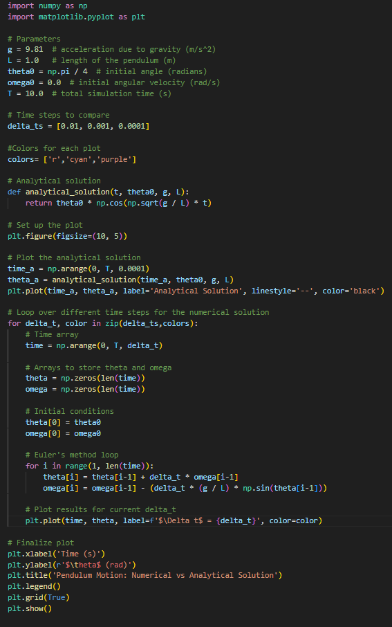
Figure 1: Code for varying \( Δt \)

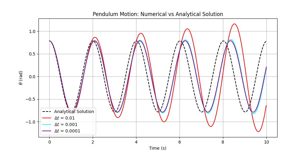
Figure 2: Plot of numerical vs analytical solution with varying \( Δt \)

From this plot, we can observe that all the numerical solutions are relatively accurate at first but begin to diverge from the analytical solution as time increases. This is due to the amplification of errors from performing Euler’s method iteratively over a longer time period. We can also observe that the error is greater for greater values of \( Δt \) , illustrating the lower degree of accuracy when using bigger timesteps. We also observe a special case in \( Δt=0.01 \) , where the angular displacement increases along with time. This is impossible due to the conservation of energy. As such, we can deduce that the numerical solution is unstable when \( Δt=0.01 \) . We can see that this is not the case when \( Δt=0.001 or 0.0001 \) , where the amplitude of the plot remains constant. This may be empirical evidence that the stability criterion for \( Δt \) lies within 0.001 and 0.0001.

Next, we varied the initial angular displacement. Fig 3 shows the code used and Fig 4 shows the resulting plot.

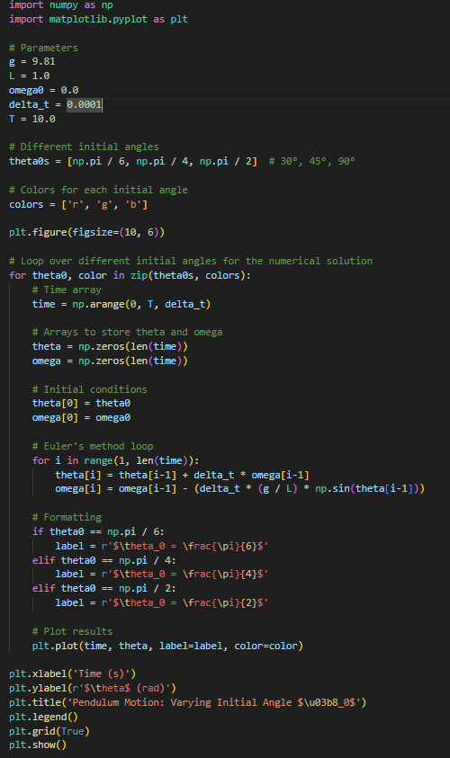
Figure 3: Code for varying \( θ \)

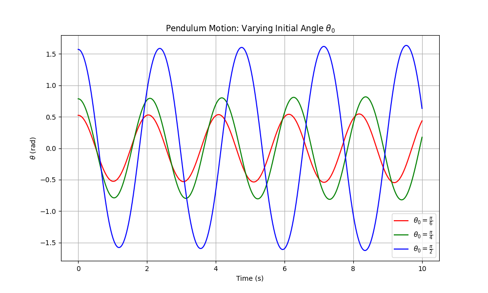
Figure 4: Plot of pendulum motion varying \( θ \)

Here, we observe that the amplitude for each plot is different as the initial angular displacement varies. However, the period remains the same as it is independent of the angular displacement. The slight phase difference observed is likely due to errors in iterating Euler’s method. The lowest timestep is used here to ensure that the solution is as accurate as possible.

Finally, we varied the pendulum length. Fig 5 shows the Python code and Fig 6 shows the plot.

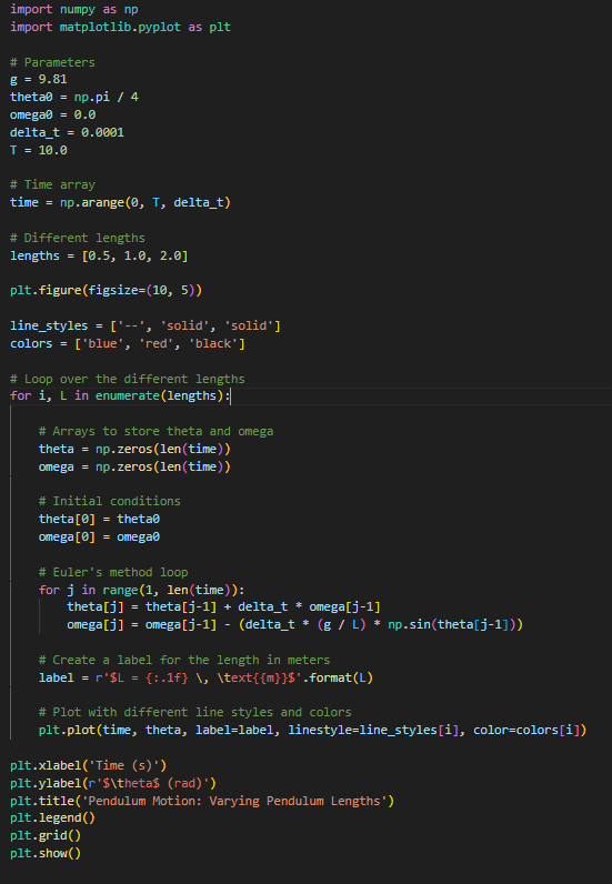
Figure 5: Code for varying \( L \)

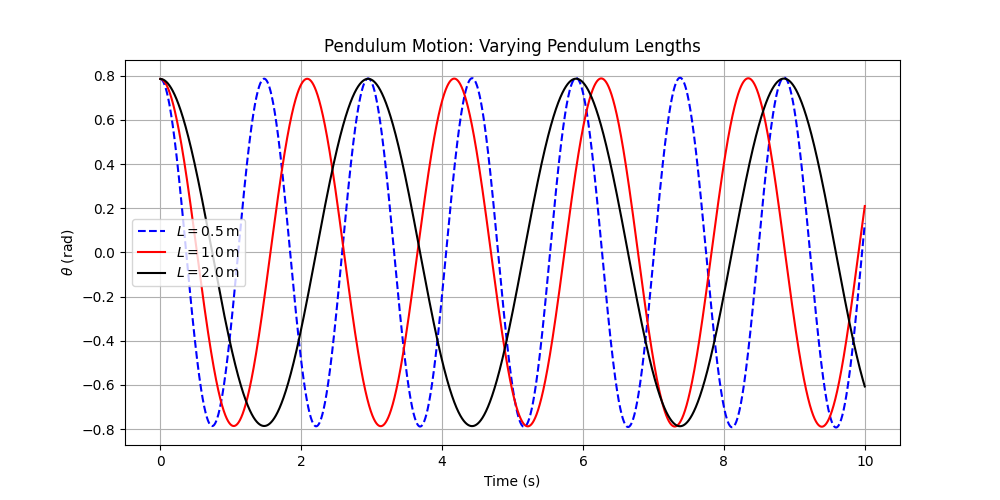
Figure 6: Plot of pendulum motion varying \( L \)

Pendulum length is a factor that affects the period of the pendulum by a factor of the square root of the length. As such, the different pendulum lengths produce different periods, while the amplitude remains the same as the initial angular displacement is constant. In particular, we observe that the period is doubled when the length is quadrupled from 0.5 to 2 meters, proving the relationship stated above.

Through the various plots, we can observe the effects of different parameters on the motion of a simple pendulum and the effects of different timesteps on the stability and accuracy of a numerical solution.

5. Conclusion

5.1. Non-uniqueness

In a word, solution non-uniqueness is a very important phenomenon in mathematical research. It enriches not only mathematical theory but also provides more possibilities for practical application. The future can further explore the use of solution diversity in different fields and how to manage and utilize this diversity effectively.

5.2. Dependence on initial conditions

These methods give a larger view of the system's dynamic characteristics and possible solutions. This is essential in developing more stable and reliable systems. In practical applications, understanding a system's non-uniqueness allows engineers and researchers to design systems that can adapt to a variety of conditions or devise strategies that can predict and control multiple behaviors.

In conducting such tests, detailed data recording and the use of appropriate statistical methods in analyzing results are necessary. This will help ensure the accuracy of the test results and provide reliable information for system design.

5.3. Numerical solution

The pendulum is a fascinating yet deceivingly simple and classical physical problem that elucidates many other areas of research. In this research, we only considered the motion of a simple pendulum – but such an ideal problem rarely exists in the real world. To further our research and make it more applicable in real life, we can introduce other elements, such as air resistance (by adding a damping constant to the differential equation), consider that the string has mass, and perhaps even how the shape of the pendulum bob may interact with air resistance and drag. These additional factors allow the motion of a pendulum to better mimic real-life phenomena, making our research more applicable and useful to real-world situations.

One big limitation in our research is the use of small angle approximation to derive a stability criterion. Small angle approximation is usually only applicable to angles smaller than 5 degrees, which greatly limits the applicability of our results. As such, our solutions may not be stable and accurate when considering larger angles. In the future, perhaps we can use other methods to achieve a more accurate numerical solution, such as the Runge-Katta method or von-Neumann stability analysis. These methods may be more accurate than Euler’s method in predicting and modeling oscillatory motion like that of a simple pendulum.

Lastly, research in pendulums can have a wide range of real-world applications other than the field of numerical modeling. Pendulums are used all over the world for a myriad of purposes – in clocks, metronomes, amusement park rides, earthquake detection, and even in astrophysics. The pendulum is truly a compelling phenomenon that impacts our world in many meaningful ways. With such a broad range of fields where we can apply our knowledge, we are extremely excited to develop our research further and grateful for the opportunity to undertake this project.

Authors contribution

Dingyu Cui: All the research on non-uniqueness in the paper;

Keni Zhang: Abstract, keywords, introduction (expect non-uniqueness), literature review;

Sean Lau: All the research on numerical solution in the paper.

References

[1]. ZOU Tong, HU Xichen, SUN Hui, GAO Jianzhi, WANG Hengtong. Theoretical Modeling and Numerical Simulation of Circular Pendulum Motion[J]. Experiment Science and Technology, 2021, 19(5): 12-17. DOI: 10.12179/1672-4550.20200363
[2]. He Guangyuan Huang Naiben. Motion equation, numerical simulation and experimental verification of spherical pendulum [J]. University Physics, 2006, 25(7): 46-46.
[3]. GuanHui [1] Li Weishan [2]. Spring pendulum motion study [J]. Journal of college physics, 2010, 29 (3) : 16-16. Results in Physics ( IF 4.4 ) Pub Date: 2021-06-13 , DOI: 10.1016/j.rinp.2021.104325 V.S. Erturk , J. Asad , R. Jarrar , H. Shanak , H. Khalilia
[4]. Huo Junrong, Zhang Rongpei. Initial value problem of differential equations based on Euler method [J]. Theoretical Mathematics, 2021, 011(008):P.1488-1492.
[5]. Feng Jianqiang, Sun Shiyi. Fourth order runge - kutta method principle and its application [J]. Journal of mathematics learning and research, 2017 (17) : 3. DOI: CNKI: SUN: SXYG. 0.2017-17-002.
[6]. Henry Guillotte, Su Dianzhen. Some Applications of Finite Difference Method [J]. Mathematics Teaching Research, 1989.
[7]. Bathe, Klaus-Jurgen. Finite Element Method: Theory, Format and Solution. 2019 edition. Upper [M]. Higher Education Press,2020.
[8]. In North-Holland Series in Applied Mathematics and Mechanics, 2003
[9]. Dependence on initial conditions, Haddow, in Encyclopedia of Vibration, 2001
[10]. Non-uniqueness of Moving Average Models, P. K. Bhattacharya, Prabir Burman, in Theory and Methods of Statistics, 2016
Cite this article
Zhang,K.;Lau,S. (2025). Numerical Modeling: Simulating the Motion of a Pendulum. Theoretical and Natural Science,107,99-110.
Data availability
The datasets used and/or analyzed during the current study will be available from the authors upon reasonable request.
Disclaimer/Publisher's Note
The statements, opinions and data contained in all publications are solely those of the individual author(s) and contributor(s) and not of EWA Publishing and/or the editor(s). EWA Publishing and/or the editor(s) disclaim responsibility for any injury to people or property resulting from any ideas, methods, instructions or products referred to in the content.
About volume
Volume title: Proceedings of the 4th International Conference on Computing Innovation and Applied Physics
© 2024 by the author(s). Licensee EWA Publishing, Oxford, UK. This article is an open access article distributed under the terms and
conditions of the Creative Commons Attribution (CC BY) license. Authors who
publish this series agree to the following terms:
1. Authors retain copyright and grant the series right of first publication with the work simultaneously licensed under a Creative Commons
Attribution License that allows others to share the work with an acknowledgment of the work's authorship and initial publication in this
series.
2. Authors are able to enter into separate, additional contractual arrangements for the non-exclusive distribution of the series's published
version of the work (e.g., post it to an institutional repository or publish it in a book), with an acknowledgment of its initial
publication in this series.
3. Authors are permitted and encouraged to post their work online (e.g., in institutional repositories or on their website) prior to and
during the submission process, as it can lead to productive exchanges, as well as earlier and greater citation of published work (See
Open access policy for details).