1. Introduction

The Monte Carlo method is an instrument that has been proven to be flexible in many applications within the financial field. For example, Frey and McNeil [1] demonstrate the technique's power in assessing credit risk by simulating Value at Risk and expected loss for credit portfolios in different economic scenarios. Similarly, Brigo and Mercurio [2] apply the Monte Carlo method to interest rate modelling, demonstrating its usefulness in complex derivative pricing and risk management assessment. In financial engineering, Glasserman [3] applies the Monte Carlo method widely in derivative pricing and hedging, where analytical solutions take time to come by. In different types of options, Boyle, Phelim, and Emanuel [4] explored the method's application in option pricing, where it was used to evaluate the values of American and European options, demonstrating its robustness across different financial instruments. Finally, Tilley [5] explored the valuation of American options using the Monte Carlo method. It offers a path-dependent method to make the valuation of options more accurate. These previous studies have shown that the applicability of the Monte Carlo method in research in the financial field is broad and valid, thus making it a significant tool for modern financial analyses.

Options are financial tools that give their holders the right but not the obligation to sell or buy an underlying asset on a certain future date at a predetermined price [6]. In our study, pricing for four forms of European options was taken into consideration. An option's value depends on several elements, including strike price, remaining time until expiration and interest rates. Accuracy is always significant in the pricing. The Monte Carlo method is coupled with financial mathematics and computer analysis. It has become an indispensable numerical tool for option pricing due to its ability to handle different options elements and wide application in complex financial models [3]. The Monte Carlo method needs several estimation processes based on many potential price paths for an option to estimate its approximate price [7]. Nevertheless, Monte Carlo simulations often require numerous samples to achieve accuracy, which needs significant computational resources [7]. To overcome these challenges, researchers have developed variance-decreasing tools, such as antithetic and control variables, that increase efficiency without compromising accuracy [8].

The Central Limit Theorem provides compelling evidence of their effectiveness in decreasing variance in work. Given a collection of independently distributed stochastic variables, this theory states that their means will resemble a normal distribution [9]. Depending on the theory, antithetic variates and control variates are often employed to reduce variance. The control variates method reduces estimates' variance by adding an auxiliary variable related to its target variable and a known expected value. Option pricing involves selecting a control variable with known relations and expectations in order to help correct estimates, thus decreasing variance. Antithetic variates is another method that reduces variance by producing negative correlation samples with symmetric properties [10]. According to the Central Limit Theorem, these samples tend to have normal distributions [9]. Antithetic variates create pairs of samples to reduce the variance and achieve accuracy with a small number of samples. Efficiency and reliability can both be achieved through these two methods.

This research explores the roles of antithetic and control variates used in Monte Carlo simulations to increase option pricing accuracy while decreasing computational time. In reality, economic benefits may come from small variance reductions. Knowledge of these methods and their usage is vital to risk management and investment decision-making within financial markets. Specifically, this research elaborates on theoretical effects related to control variates and antithetic variates for Monte Carlo simulations while conducting numerical experiments to test impacts and provide practical guidelines that may assist both theoretical research and real-world operations.

2. Methodology

2.1. Introduction

In the following part, two optimized methods will be introduced: the control variates method and the antithetic variable method. The control variates method decreases the variance by adding an auxiliary variable, while the antithetic variable method decreases the variance by creating pairs of samples. In the final part, the parameters l and m will be introduced, indicating the optimized effect of the two methods above.

2.2. Optimized method of Monte-Carlo methods

According to the Black-Scholes Model, S(T), which indicates the stock price at time T, is given as follows:

\( S(T)=S(0)exp((r-\frac{{σ^{2}}}{2})T+σ\sqrt[]{T}Z) \) ,(1)

where Z has the standard normal distribution and σ is a parameter representing the stock’s ’volatility’.

Suppose the result is to calculate the price of a European call whose payoff is \( {(S(T)-K)^{+}} \) . Then, a random variable can be defined.

\( X={e^{-rT}}{(S(T)-K)^{+}} \) .(2)

Since \( E[{e^{-rT}}S(T)]=S(0) \) . This yields \( E[S(T)]={e^{-rT}}S(0) \) . Then, the price \( V(0) \) of a call option with strike K can be computed as

\( V(0)={e^{-rT}}E[{(S(T)-K)^{+}}] \) (3)

A row of i.i.d random numbers, \( {X_{i}} \) , would be created, whose distribution equals the distribution of \( X \) . Then, according to the strong law of large numbers, \( E[{(S(T)-K)^{+}}] \) can be estimated as \( \frac{1}{n}\sum _{j=1}^{n}{X_{j}} \) . This method is called the Monte Carlo method.

In this essay, the work is to compare the rate of convergence of original Monte-Carlo methods with the rate of optimized Monte-Carlo methods.

2.2.1. Control variates method

The idea of using control variates

A sequence \( ({X_{i}},{ Y_{i}}) \) of i.i.d. random vectors from the joint distribution of \( (X, Y) \) (where we know \( E[Y] \) ) can be defined as:

\( {X_{i}}(b)={X_{i}}-b({Y_{i}}-E[Y]),for i=1,2,..., \) (4)

where \( b∈R \) is a constant (R stands for the real numbers).

Whatever value b takes, \( ({X_{i}}(b)) \) is a sequence of random variables such that

\( E[{X_{i}}(b)]=E[{X_{i}}]-b(E[{Y_{i}}]-E[Y])=E[X]; \)

\( Var({X_{i}}(b))=Var({X_{i}}-b{Y_{i}}) \) (5)

\( =Var(x)-2bCov(X,Y)+{b^{2}}Var(Y). \)

Note that \( \bar{{Y_{n}}}-E[Y] \) is used to control the estimation of \( E[X] \) .

The mean of the control-variates estimator is

\( E[\bar{{X_{n}}}(b)]=\frac{1}{n}\sum _{i=1}^{n}E[{X_{i}}(b)]=E[X], \) (6)

so it is unbiased.

The control-variates estimator's variance is

\( Var(\bar{{X_{n}}}(b))=\frac{1}{{n^{2}}}\sum _{i=1}^{n}Var{(X_{i}}(b)) \) (7)

\( =\frac{1}{n}Var{(X_{i}}(b) \) (8)

\( =\frac{1}{n}(Var(X)-2bCov(X,Y)+{b^{2}}Var(Y)) \) (9)

This variance is a function in \( b \) , and we want to minimize it with respect to \( b \) .

By setting the derivative in \( b \) equal to zero, we can get the value b^∗ , which minimizes the variance \( Var(\bar{{X_{n}}}(b)) \) . This value is given by

\( {b^{*}}=\frac{Cov(X,Y)}{Var(Y)} \) (10)

Substituting \( {b^{*}} \) for \( b \) in \( (9) \)

\( Var(\bar{{X_{n}}}({b^{*}}))=\frac{1}{n}(Var(X)-\frac{{Cov(X,Y)^{2}}}{Var(Y)}). \) (11)

This expression and the fact that

\( Var(\bar{{X_{n}}})=\frac{1}{n}Var(X) \) (12)

Imply that

\( \frac{Var(\bar{{X_{n}}}({b^{*}}))}{Var(\bar{{X_{n}}})}=1-\frac{{Cov(X,Y)^{2}}}{Var(Y)}=1-2_{ρ}^{XY}, \) (13)

where \( {ρ_{XY}} \) is the correlation coefficient between \( X \) and \( Y \) .

When the squared correlation \( 2_{ρ}^{XY} \) of \( X \) and Y is large, and it is easy to generate the samples, Yi, the control-variates method is useful.

If \( E[X] \) is unknown and we need Monte Carlo to estimate it, then it is quite possible that \( Cov(X, Y) \) is unknown.

To continue to estimate, an unbiased estimator \( \hat{n_{*}^{b}} \) of \( {b^{*}} \) can be used.

In particular, set

\( \hat{*_{b}^{n}} =\frac{\sum _{i=1}^{n}({X_{i}}-\bar{{X_{n}}})({Y_{i}}-\bar{{Y_{n}}})}{\sum _{i=1}^{n}{({Y_{i}}-\bar{{Y_{n}}})^{2}}} \) .(14)

The control-variates estimator mentioned above is given by \( \frac{1}{n}\sum _{i=1}^{n}{X_{i}}(\hat{*_{b}^{n}} ) \) , where

\( {X_{i}}(\hat{*_{b}^{n}})={X_{i}}-\frac{\sum _{i=1}^{n}({X_{i}}-\bar{{X_{n}}})({Y_{i}}-\bar{{Y_{n}}})}{\sum _{i=1}^{n}{({Y_{i}}-\bar{{Y_{n}}})^{2}}} ({Y_{i}}-E[Y]) \) .(15)

\( Y \) in the call price estimator equals to \( S(T) \) , and \( X \) in the call price estimator equals to \( {e^{-rT}}{(S(T)-K)^{+}} \) .

2.2.2. Antithetic variable method

To decrease the variance of the estimate, we can use the \( \frac{1}{2}(h({x_{1}})+h(-{x_{1}})) \) to replace the \( \frac{1}{2}(h({x_{1}})+h({x_{2}})) \) .

\( Since Var(\frac{1}{2}(h({x_{1}})+h(-{x_{1}}))-Var(\frac{1}{2}(h({x_{1}})+h({x_{2}}))=Cov(h({x_{1}}),h(-{x_{1}})), if Cov(h({x_{1}}),h(-{x_{1}})) \lt 0 \) , the rate of convergence can be improved by using the antithetic variable.

2.3. connection between the rate of convergence and K

Let \( l=2_{ρ}^{XY} \)

\( l \) is a parameter indicating the effect of control variates, which shows that the effect is better when \( l \) is bigger. By plotting the image with K as the x-axis and \( l \) as the y-axis, a conclusion can be got that the effect of improvement of control-variates decreases by the increase of K. It is really hard to prove the conclusion above directly by math, but it may be proved intuitively. According to:

\( Y=S(T),X={e^{-rT}}{(S(T)-K)^{+}} \) (16)

When \( K=0 \) , \( X={e^{-rT}}S(T) \) , which is highly correlated with \( Y \) . Then \( l \) can reach the maximal 1. With \( K \) increasing, the correlation between X and Y is lower and lower. Thus, l will go down meanwhile. Next, let

\( m=1-\frac{Var(\frac{1}{2n}\sum _{i=1}^{n}h({x_{i}})+h(-{x_{i}}))}{Var(\frac{1}{2n}\sum _{i=1}^{n}h({x_{i}}))} \) (17)

m is a parameter indicating the effect of the antithetic variable, which shows that the effect is better when \( l \) is bigger.

By plotting the image with K as the x-axis and m as the y-axis, the effect of improvement of the antithetic variable first decreases by the increase of K, and when K reach some value, the effect begins increasing with K increasing.

2.4. Using Monte-Carlo technics to predict prices of other options

(1) For the put option: let \( X={e^{rT}}{(K-S(T))^{+}} \)

(2) For the power option: let \( X={e^{rT}}S(T) \)

(3) For the log option: let \( X={e^{rT}}logS(T) \)

3. Results

This work compared the variance optimization effects of Monte Carlo simulation using control variates and antithetic variates in the pricing of call options, put options, power options and log options based on the given indicators (see Table 1).

Table 1: Parameters

Note. r is the risk-free rate

In Fig.1, the green line represents a standard Monte Carlo; the blue line represents Monte Carlo simulation based on control variables; the orange line represents Monte Carlo based on antithetic variables; and the red line represents the true value. The horizontal and vertical axes represent the sample size and option price, respectively. According to the law of large numbers, the more samples there are, the closer the probability is to the expected value. In call options, compared to the standard Monte Carlo, the optimized Monte Carlo has a faster convergence rate.

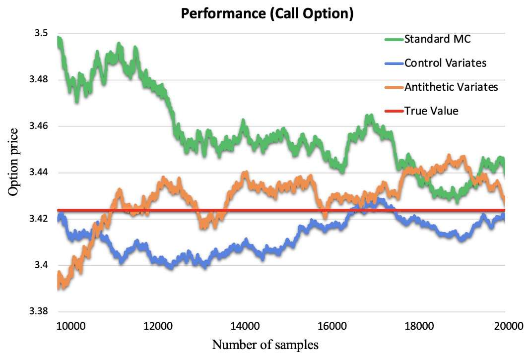
Figure 1: Performance of Monte-Carlo in call options

This work calculated the variance optimization effects of the control variable and antithetic variable on standard Monte Carlo estimation under different strike K values. As Fig.2 shows, when K is small, the control variable has a slight advantage over the antithetic variates, while when K is large, the antithetic variates have a better optimization effect.

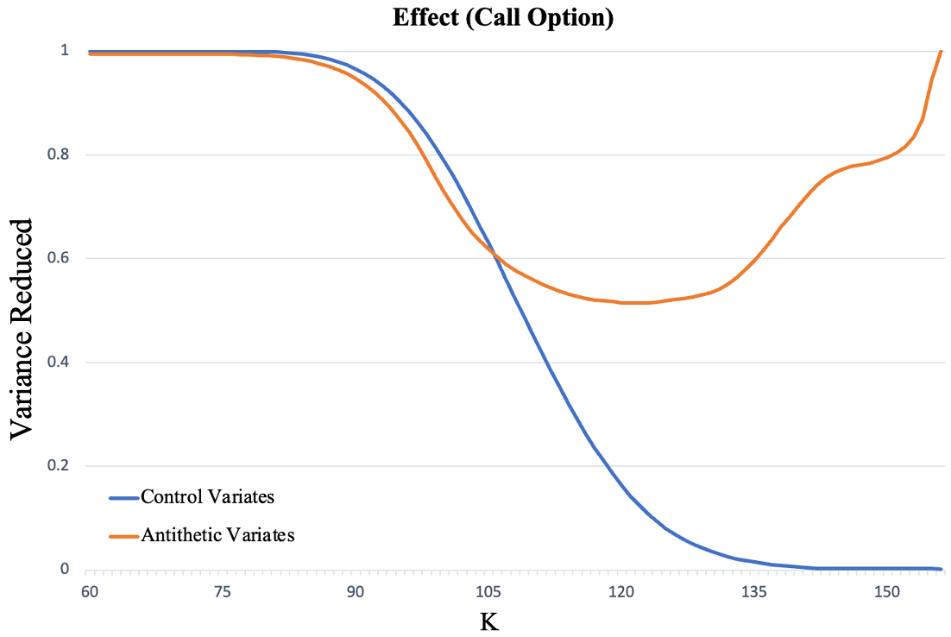
Figure 2: Optimization effect of variance

These two lines cross at K=106, and the variance reduced at this point is 62%. From the overall effect, for call options, Monte Carlo optimized by using antithetic variates reduces the variance by about 80% in option pricing compared to ordinary Monte Carlo, outperforming Monte Carlo simulations based on control variables.

Next, we extend our calculations to put options. Fig.3(a) shows that the optimized Monte Carlo also has faster convergence rate input options. Moreover, Fig.3(b) illustrates that Monte Carlo based on antithetic variables is always better than Monte Carlo based on control variables input options.

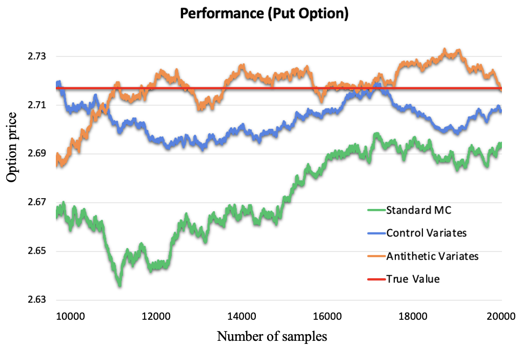
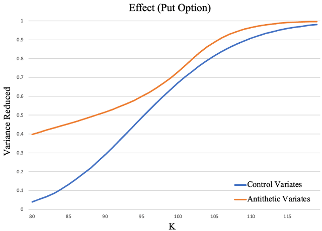
(a) (b)

Figure 3: Performance of Monte-Carlo input options

As Fig.4(a) shows, Monte Carlo based on antithetic variables performs particularly well in the log option, which completely cancels the variance. The green line representing the antithetic variates is a straight line. It is because, in this case, the formula changes into

\( Y={e^{-rT}}(ln{S_{0}}+(r-0.5{σ^{2}})T) \) (18)

Since \( r \) , \( σ \) , \( T \) and \( {S_{0}} \) are both known terms, Y is a constant value. The variance of Y is 0.

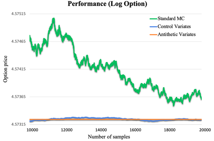
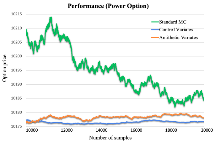
(a) (b)

Figure 4: Performance of Monte-Carlo in log & power options

Table 2: Optimization Effect

As Fig.4(b) shows, for power options, control variates seem better. From Table 2, the variance of Monte Carlo simulation using Control variates (0.006* \( {V_{standardMC}} \) ) is less than one-third of that using antithetic variates (0.021* \( {V_{standardMC}} \) ).

4. Conclusion

In most cases, the Monte Carlo optimization based on antithetic variates performs well. Compared to standard Monte Carlo, Monte Carlo optimized with antithetic variates effectively reduces the variance of option prices and provides more accurate estimates of option prices. However, using control variates to optimize Monte Carlo still needs to be considered, as it has shown surprising results in certain options, such as power options.

In the future, we are considering building the model on this basis and extending its perceptual capabilities to collect real-time stock and option prices, use different Monte Carlo variants for option pricing, and design trading strategies for different options.

References

[1]. Frey, R. and McNeil, A.J. (2002) ‘Var and expected shortfall in portfolios of Dependent Credit Risks: Conceptual and practical insights’, Journal of Banking & Finance, 26(7), pp. 1317–1334. doi:10.1016/s0378-4266(02)00265-0.
[2]. Brigo, D. & Mercurio, F. (2006) ‘Interest rate models : theory and practice : with smile, inflation, and credit’. Second edition. Berlin: Springer
[3]. Glasserman, P. (2003) ‘Monte Carlo Methods in financial engineering’, Stochastic Modelling and Applied Probability [Preprint]. doi:10.1007/978-0-387-21617-1.
[4]. Boyle, P.P. (1977) 'Options: A Monte Carlo approach’, Journal of Financial Economics, 4(3), pp. 323–338. doi:10.1016/0304-405x(77)90005-8.
[5]. Tilley, J.A. (1993) ‘Valuing American options in a path simulation model’, Insurance: Mathematics and Economics, 16(2), p. 169.doi:10.1016/0167-6687(95)91768-h.
[6]. Sayan, M. (2023) ‘Options’, The Palgrave Encyclopedia of Islamic Finance and Economics, pp. 1–7. doi:10.1007/978-3-030-93703-4294-1.
[7]. Kailash C., P., Raouf, G. and Funmilayo Eniola, K. (2015) Multilevel Monte Carlo simulation in options pricing, University of Western Cape. University of the Western Cape. Available at: http://hdl.handle.net/11394/4349.
[8]. Boyle, P., Broadie, M. and Glasserman, P. (1997) ‘Monte Carlo methods for security pricing’, Journal of Economic Dynamics and Control, 21(8–9), pp. 1267–1321. doi:10.1016/s0165-1889(97)00028-6.
[9]. Kwak, S.G. and Kim, J.H. (2017) ‘Central limit theorem: The cornerstone of modern statistics’, Korean Journal of Anesthesiology, 70(2), p.144. doi:10.4097/kjae.2017.70.2.144.
[10]. Kwon, C. and Tew, J.D. (1994) ‘Strategies for combining antithetic variates and control variates in designed simulation experiments’, Management Science, 40(8), pp. 1021–1034. doi:10.1287/mnsc.40.8.1021.
Cite this article
Mo,Z.;He,B.;Qin,T. (2025). Option Pricing Based on Several Monte Carlo Techniques. Theoretical and Natural Science,107,227-234.
Data availability
The datasets used and/or analyzed during the current study will be available from the authors upon reasonable request.
Disclaimer/Publisher's Note
The statements, opinions and data contained in all publications are solely those of the individual author(s) and contributor(s) and not of EWA Publishing and/or the editor(s). EWA Publishing and/or the editor(s) disclaim responsibility for any injury to people or property resulting from any ideas, methods, instructions or products referred to in the content.
About volume
Volume title: Proceedings of the 4th International Conference on Computing Innovation and Applied Physics
© 2024 by the author(s). Licensee EWA Publishing, Oxford, UK. This article is an open access article distributed under the terms and
conditions of the Creative Commons Attribution (CC BY) license. Authors who
publish this series agree to the following terms:
1. Authors retain copyright and grant the series right of first publication with the work simultaneously licensed under a Creative Commons
Attribution License that allows others to share the work with an acknowledgment of the work's authorship and initial publication in this
series.
2. Authors are able to enter into separate, additional contractual arrangements for the non-exclusive distribution of the series's published
version of the work (e.g., post it to an institutional repository or publish it in a book), with an acknowledgment of its initial
publication in this series.
3. Authors are permitted and encouraged to post their work online (e.g., in institutional repositories or on their website) prior to and
during the submission process, as it can lead to productive exchanges, as well as earlier and greater citation of published work (See
Open access policy for details).