1. Introduction

Pendulum motion has been a basic component of classical mechanics, providing a lot of research opportunities as an effective teaching tool. Since the late 16th century, pendulums have captivated the attention of scientists. This research is important for its historical background as its potential applications in a different field, including robotics, aerospace engineering, and seismology.

The two ways we use to modelling the motion of a pendulum are the analytical and numerical methods. The analytical method uses Newton's law to create equations that can explain the pendulums under ideal conditions motion, while the numerical method uses computer technology to find solutions in harder scenarios, such as air resistance and wider angles of oscillation. In Section 2, the strengths and disadvantages of the numerical and analytical approaches will be compared and contrasted. Section 3 will examine the relationship between angle and time in pendulum motion. The addition of air resistance to pendulum dynamics will be covered in Section 4. Section 5 presents the double pendulum system. The last sections will compare our findings and conclusions.

2. Numerical methods and analytical methods

The pendulum is made of one mass \( m \) is suspended on a massless string of length l, and the Angle change is an essential research factor in the process of exploring the motion of the pendulum. In order to study the close relationship between numerical and analytical methods, this research use the relationship between the change of research Angle ( \( θ \) ) and time ( \( t \) ) to make an intuitive comparison.

Assuming that the pendulum oscillates at a small angle and ignores the air resistance, so the study constructs a harmonic motion model. Newton's laws are shown in Eq. 1 [1,2],

\( \sum τ=Iα\ \ \ （1） \)

where \( τ \) is torque, \( I \) is moment of inertia, and \( α \) is angular acceleration [3]. Torque can be expressed as \( τ=Fr \) , and r is the distance from F to the axis point. The moment of inertia can be likened to the mass m, and the moment of inertia of a particle is \( I=m{r^{2}} \) . Angular acceleration measures the change in angular velocity \( ω \) .

According to \( τ=Fr \) , in this case \( r=l \) , \( F=mgsin{θ} \) , derived from the decomposition of forces. Then substitute \( I=m{r^{2}} \) by equal quantity, and combine Eq. 1 to get the equivalent expression.

\( -lmgsin{θ}=m{l^{2}}α\ \ \ (2) \)

To simplify and rearrange,

\( -\frac{g}{l}sin{θ}=α\ \ \ (3) \)

For simplicity, it uses \( ω=\sqrt[]{\frac{g}{l}} \) [3]. Since angular acceleration is the second derivative with respect to time, \( α=\frac{{d^{2}}θ}{d{t^{2}}} \) . Then get the differential equation of simple pendulum motion,

\( \frac{{d^{2}}θ}{d{t^{2}}}=-{ω^{2}}sin{θ}.\ \ \ (4) \)

Since the condition this study sets before is a small Angle pendulum, \( sin{θ}≈θ \) , the error in the middle is negligible. Using the first important limit theorem [4],

\( \underset{θ→0}{lim}{\frac{sin{θ}}{θ}}=1\ \ \ (5) \)

Get,

\( \frac{{d^{2}}θ}{d{t^{2}}}≈-{ω^{2}}θ.\ \ \ (6) \)

Therefore, reducing Eq. 4 to Eq. 6. To solve this differential equation, this study notes that the second order differential equation satisfies the form of the second order linear homogeneous differential equation [5], so this study sets \( θ={e^{iωt}} \) to find the first and second derivatives [3],

\( θ={e^{iωt}}\ \ \ （7） \)

\( \frac{dθ}{dt}=iω{e^{iωt}}\ \ \ （8） \)

\( \frac{{d^{2}}θ}{d{t^{2}}}=-{ω^{2}}{e^{iωt}}=-{ω^{2}}θ.\ \ \ （9） \)

So, the study indicates that \( θ={e^{iωt}} \) is the solution to the second order differential equation in Eq. 6, so it uses \( {θ_{1}}={C_{1}}{e^{iωt}} \) , \( {θ_{2}}={C_{2}}{e^{-iωt}} \) , \( {C_{1}}{C_{2}}∈C \) [3],

\( θ={C_{1}}{e^{iωt}}+{C_{2}}{e^{-iωt}}\ \ \ （10） \)

Take one derivation and it gets,

\( \frac{dθ}{dt}={C_{1}}iω{e^{iωt}}-{C_{2}}{iωe^{-iωt}}\ \ \ （11） \)

And then taking the derivative again and getting,

\( \frac{{d^{2}}θ}{d{t^{2}}}={-C_{1}}{ω^{2}}{e^{iωt}}+{C_{2}}{{ω^{2}}e^{-iωt}} \)

\( =-{ω^{2}}({C_{1}}{e^{iωt}}+{C_{2}}{e^{-iωt}}) \)

\( =-{ω^{2}}θ.\ \ \ (12) \)

Thus, Eq. 12 satisfies Eq. 6 and contains all possible solutions. Applying Euler's formula \( {e^{ix}}=cos{x}+isin{x} \) to this general solution [3], get,

\( θ={C_{1}}cos{ωt}+{C_{1}}isin{ωt}+{C_{2}}cos{(-ωt)}+{C_{2}}isin{(-ωt).}\ \ \ (13) \)

Since \( sin{(-θ)}=-sin{θ} \) , \( cos{(-θ)}=-cos{θ} \) ,

\( θ={C_{1}}cos{ωt}+{C_{1}}isin{ωt}+{C_{2}}cos{(ωt)}-{C_{2}}isin{(ωt).}\ \ \ (14) \)

After rearranging,

\( θ=({C_{1}}+{C_{2}})cos{ωt}+i({C_{1}}-{C_{2}})sin{ωt}\ \ \ (15) \)

Then let \( A={C_{1}}+{C_{2}} \) , \( B=i({C_{1}}-{C_{2}}) \) [3],

\( θ=Acos{ωt}+Bsin{ωt}\ \ \ (16) \)

This formula is a continuous function to study the relationship between Angle change and time in simple pendulum motion, in which analytical method is used. In this formula, \( A,B∈R \) is the constant of the initial condition of a simple pendulum. Now thinking about the approximation equation.

Using linear approximation to define the first derivative,

\( \frac{dθ}{dt}≈\frac{{θ_{i}}-{θ_{i-1}}}{∆t}\ \ \ (17) \)

By analogy, applied to the second derivative approximation,

\( \frac{{d^{2}}θ}{d{t^{2}}}≈\frac{{θ_{i}}-{θ_{i-1}}}{∆t}{|_{i+1}}-\frac{{θ_{i}}-{θ_{i-1}}}{∆t}{|_{i}} \)

\( ≈\frac{1}{∆t}(\frac{{θ_{i+1}}-{θ_{i}}}{∆t}-\frac{{θ_{i}}-{θ_{i-1}}}{∆t}) \)

\( =\frac{{θ_{i+1}}-2{θ_{i}}+{θ_{i-1}}}{∆{t^{2}}}\ \ \ (18) \)

According to Eq. 3,

\( \frac{{d^{2}}θ}{d{t^{2}}}=-\frac{g}{l}sin{{θ_{i}}}\ \ \ (19) \)

Therefore, the approximate equation can be obtained according to Eq. 18 and Eq. 19.

\( \frac{{θ_{i+1}}-2{θ_{i}}+{θ_{i-1}}}{∆{t^{2}}}=-\frac{g}{l}sin{{θ_{i}}}\ \ \ （20） \)

Now let us consider the air resistance conditions; first of all, only one resistance----the air resistance \( {F_{1}} \) applied to the ball. Since the resistance \( {F_{1}} \) is opposite to the direction of motion and proportional to the velocity of motion, this research defines the resistance as a function of velocity.

\( {F_{1}}=-kv\ \ \ （21） \)

In the rotation motion, the angular velocity \( ω=\frac{v}{r} \) , \( v=rω \) , where r is the distance from the moving particle to the axis point, \( r=l \) . So, this study gets, on the basis of Eq. 21,

\( {F_{1}}=-klω\ \ \ (22) \)

Next, the study applies Newton's laws,

\( \sum F=ma\ \ \ (23) \)

Where \( a \) is the linear acceleration, and in the rotation motion, \( a=rα \) , so this study can get,

\( mlα=-mgsin{θ}-klω \)

\( =-mgθ-klω\ \ \ (24) \)

Because \( α=\frac{{d^{2}}θ}{d{t^{2}}} \) , this research gets,

\( ml\frac{{d^{2}}θ}{d{t^{2}}}=-mgθ-kl\frac{dθ}{dt}\ \ \ (25) \)

For simplify,

\( \frac{{d^{2}}θ}{d{t^{2}}}+\frac{k}{ml}\frac{dθ}{dt}+\frac{g}{l}θ=0\ \ \ (26) \)

Now it defines a constant \( γ=\frac{k}{ml} \) ,

\( \frac{{d^{2}}θ}{d{t^{2}}}+γ\frac{dθ}{dt}+\frac{g}{l}θ=0\ \ \ (27) \)

This research indicates that Eq. 27 satisfies homogeneous second order linear differential equation with constant coefficient, so this research can get the general solution [6],

\( θ={e^{-γt}}(Acos{ωt}+Bsin{ωt})\ \ \ (28) \)

Where \( γ \) is constant, \( ω={{ω_{0}}^{2}}-{γ^{2}} \) . This gives us a continuous function of a simple pendulum motion with air resistance.

Next, to consider the definition of the approximate equation, this study once again starts from the equation of Newton's law Eq. 1 of rotational motion and Eq. 24,

\( -mglsin{θ}-klv=m{l^{2}}α\ \ \ (29) \)

To simplify,

\( \frac{{d^{2}}θ}{d{t^{2}}}=-\frac{g}{l}sin{θ}+\frac{k}{ml}v \)

\( =-\frac{g}{l}sin{θ}+\frac{k}{m}ω\ \ \ (30) \)

For simplicity, the research defines a constant \( β=\frac{k}{m} \) , and since \( ω=\frac{dθ}{dt} \) , it gets,

\( \frac{{d^{2}}θ}{d{t^{2}}}=-\frac{g}{l}sin{θ}+β\frac{dθ}{dt}\ \ \ (31) \)

According to Eq. 17 and Eq. 18, the study therefore obtains the approximate equation,

\( \frac{{θ_{i+1}}-2{θ_{i}}+{θ_{i-1}}}{∆{t^{2}}}=-\frac{g}{l}sin{{θ_{i}}}+β\frac{{θ_{i}}-{θ_{i-1}}}{∆t}\ \ \ (32) \)

3. The relationship between angle change and time

To further investigate the close connection between the pendulum Angle change and the time change, considering a slightly more complicated case: on the basis of the air resistance \( {F_{1}} \) , this study considers the air resistance \( {F_{2}} \) applied to the rope.

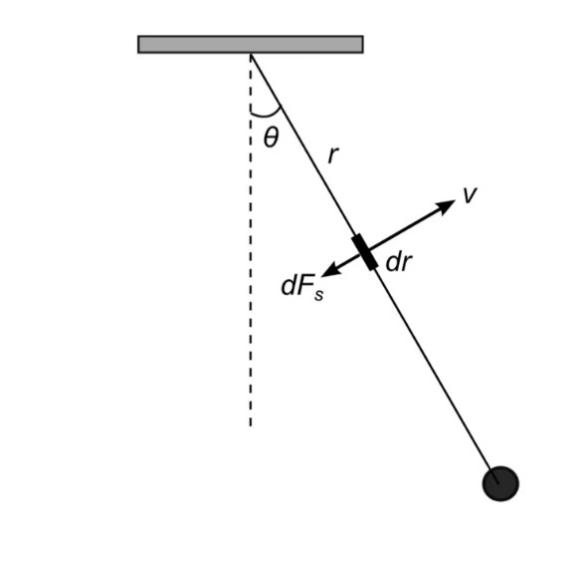
Figure 1: Force analysis of simple pendulum with resistance on rope [6]

Figure 1 is a force analysis of a simple pendulum that experiences resistance not only from itself, but also from the rope. Considering an element of the pendulum string with length \( dr \) , located at a distance \( r \) from the support point and moving with velocity \( v \) [6]. The magnitude of the drag force on this element of the string is \( d{F_{s}} \) [6] which is \( d{F_{2}} \) in the following page.

According to Figure 1, it can be known the cross-section is proportional to the resistance [6] and Eq. 21, the study gets,

\( d{F_{2}}=c(Ddr)v\ \ \ (33) \)

Where \( D \) is the diameter of the string and \( c \) is a constant. According to \( v=rω \) , it gets,

\( d{F_{2}}=cDωrdr\ \ \ (34) \)

According to Eq. 1,

\( d{τ_{2}}=rd{F_{2}}=cDω{r^{2}}dr\ \ \ (35) \)

To solve this equation, the study takes the integral on both sides of the equal sign [6], and it gets,

\( {τ_{2}}=cDω\int _{0}^{l}{r^{2}}dr \)

\( =\frac{c{l^{3}}D}{3}ω\ \ \ (36) \)

According to Eq. 1 and Eq. 22,

\( m{l^{2}}α=-mglsin{θ}-\frac{c{l^{3}}D}{3}ω-k{l^{2}}ω\ \ \ (37) \)

So, this simplifies to,

\( α+(\frac{clD}{3m}+\frac{k}{m})ω+\frac{g}{l}sin{θ}=0\ \ \ (38) \)

Assuming a constant \( φ=\frac{clD}{3m}+\frac{k}{m} \) [6], the equation is derived,

\( α+φω+\frac{g}{l}sin{θ}=0\ \ \ （39） \)

Eq. 39 satisfies the form of homogeneous second order linear differential equation with constant coefficient [6], so this research can get the general solution,

\( θ={e^{\frac{-φt}{2}}}[Acos{ωt}+Bsin{ωt}]\ \ \ (40) \)

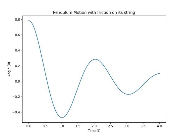
Figure 2: The relationship between angle and time of pendulum with friction on its rope

In Figure 2, the horizontal coordinate represents the time in seconds. The vertical coordinate represents the radian Angle, perpendicular to the horizontal line represents the Angle of 0, the vertical line right represents the positive Angle value, the vertical line left represents the negative Angle value.

Figure 2 represents the change of angle according to time when there exists friction on the rope of the pendulum. Because friction impedes the motion of the pendulum, the mechanical energy of the system consisting of the pendulum is getting smaller and smaller under the influence of friction [2]. The biggest angle it can achieve during each period is also getting smaller and smaller, which is represented by Figure 2.

4. The relationship between initial angle and period(T)

In order to explore the motion model of the periodic pendulum, the oscillation period is an indispensable research direction. To clarify the relationship between the initial angle and period(T), this study still starts with the simplest condition - a small-angle pendulum without air resistance.

It continues its previous research on the relationship between Angle (θ) change and time (t) by using the formula,

\( T=\frac{2π}{ω}\ \ \ (41) \)

So, with \( ω=\sqrt[]{\frac{g}{l}} \) , this study has a very simple formula for the period,

\( T=2π\sqrt[]{\frac{l}{g}}\ \ \ (42) \)

\( =mgl(1-cos{{θ_{0}}})\ \ \ (43) \)

According to Eq. 42 [3], it can intuitively see that \( T \) is constant and is independent of the initial Angle \( (θ) \) . In order to further explore the relationship between the two variables, this study changes the condition to large-angle pendulum without air resistance.

Where \( {E_{k}} \) is kinetic energy, \( {E_{p}} \) is potential energy, \( E \) is initial mechanical energy, and \( {θ_{0}} \) is initial Angle. According to Eq. 43, the equation is solved.

\( \frac{1}{2}m{l^{2}}{ω^{2}}=mgl(cos{θ}-cos{{θ_{0}}})\ \ \ （44） \)

Using this formula to solve for the angular velocity,

\( ω=\sqrt[]{\frac{2g}{l}(cos{θ}-cos{{θ_{0}}})}\ \ \ (45) \)

Replace \( ω \) with \( \frac{dθ}{dt} \) , and separate the variables,

\( \sqrt[]{\frac{2g}{l}}dt=\frac{dθ}{\sqrt[]{(cos{θ}-cos{{θ_{0}}})}}\ \ \ (46) \)

Integrating both sides: Notice the symmetry of the four phases of motion in a complete period (swing angle: from \( {θ_{0}}→0→{-θ_{0}}→0→{θ_{0}} \) ). This is why the research employed the coefficient 4 here.

\( \int _{0}^{T}\sqrt[]{\frac{2g}{l}}dt=4\int _{0}^{{θ_{0}}}\frac{dθ}{\sqrt[]{(cos{θ}-cos{{θ_{0}}})}}\ \ \ (47) \)

Applying the following trigonometric identities,

\( cos{θ}=1-2{sin^{2}}{\frac{θ}{2}}\ \ \ (48) \)

Substitute this identity into Eq. 47,

\( T=2\sqrt[2]{2}\sqrt[]{\frac{l}{g}}\int _{0}^{{θ_{0}}}\frac{dθ}{\sqrt[]{(2{sin^{2}}{\frac{θ}{2}}-2{sin^{2}}{\frac{{θ_{0}}}{2}})}}\ \ \ (49) \)

Now, try to substitute \( θ \) by \( b \) , \( b \) is an angle, assuming the relationship is,

\( sin{\frac{θ}{2}}=sin{\frac{{θ_{0}}}{2}}sin{b}\ \ \ (50) \)

Then the study takes the derivative of b with respect to theta on both sides, employ the skill differential implicitly,

\( \frac{1}{2}cos{\frac{θ}{2}}=sin{\frac{{θ_{0}}}{2}}cos{b}\frac{db}{dθ}\ \ \ （51） \)

Moving the numerators and denominator and represent \( dθ \) in terms of \( db \) ,

\( dθ=\frac{2sin{\frac{{θ_{0}}}{2}}cos{b}}{cos{\frac{θ}{2}}}db\ \ \ (52) \)

Then finding the boundary values by considering the points when the swing angle, \( θ \) , is at its minimum and maximum point ( \( 0 \) and \( { θ_{0}} \) ,respectively): When \( θ=0 \) , \( b=0 \) . When \( θ={ θ_{0}} \) , \( b=\frac{π}{2} \) . And according to Eq. 50, this study gets,

\( 2{sin^{2}}{\frac{θ}{2}}=2{sin^{2}}{\frac{{θ_{0}}}{2}}{sin^{2}}{b}\ \ \ (53) \)

After all the substitution and simplification, it has,

\( T=4\sqrt[]{\frac{l}{g}}\int _{0}^{\frac{π}{2}}\frac{db}{cos{\frac{θ}{2}}}\ \ \ (54) \)

Notice that,

\( cos{\frac{θ}{2}}=\sqrt[]{1-{sin^{2}}{\frac{{θ_{0}}}{2}}{sin^{2}}{b}}\ \ \ (55) \)

So,

\( T=4\sqrt[]{\frac{l}{g}}\int _{0}^{\frac{π}{2}}\frac{db}{\sqrt[]{1-{sin^{2}}{\frac{{θ_{0}}}{2}}{sin^{2}}{b}}}\ \ \ (56) \)

To simplify the equation, the research assumes that \( y={sin^{2}}{\frac{{θ_{0}}}{2}} \) , Substituting \( a \) into Eq. 56 [3], and define a \( Y(y) \) function, \( Y(y)=\int _{0}^{\frac{π}{2}}\frac{db}{\sqrt[]{1-{y^{2}}{sin^{2}}{b}}} \) , it gets,

\( T=4\sqrt[]{\frac{l}{g}}Y(y)\ \ \ (57) \)

Expanding \( Y(y) \) into a Maclaurin Series. This study first expands the integrated function in \( Y(y) \) (called \( f(y) \) , \( f(y)=\frac{1}{\sqrt[]{1-{y^{2}}{sin^{2}}{b}}} \) ), into a Maclaurin series and then does integration on each term. The study lets \( {y^{2}} \) = \( X \) , and expands \( f(X) \) into the Maclaurin series, it has (by definition),

\( f(X)=\sum _{i=0}^{∞}\frac{{f^{(i)}}(0)}{i!}{X^{i}} \)

\( =f(y)≈f(0)+\frac{{f^{ \prime }}(0)X}{1!}+\frac{{f^{ \prime \prime }}(0){X^{2}}}{2!}+\frac{{f^{ \prime \prime \prime }}(0){X^{3}}}{3!}+…\ \ \ (58) \)

Now substitute \( {k^{2}} \) back into the Eq. 58 and find the derivative of each term with respect to \( f \) , it obtains,

\( f(y)≈1+\frac{1}{2}{sin^{2}}{b}{y^{2}}+\frac{3}{8}{sin^{4}}{b}{y^{4}}+\frac{5}{16}{sin^{6}}{b}{y^{6}}+…\ \ \ (59) \)

The research then substitutes Eq. 59 into Eq. 57 and gets,

\( T=4\sqrt[]{\frac{l}{g}}Y(y) \)

\( =4\sqrt[]{\frac{l}{g}}\int _{0}^{\frac{π}{2}}f(y)db \)

\( =4\sqrt[]{\frac{l}{g}}\int _{0}^{\frac{π}{2}}(1+\frac{1}{2}{sin^{2}}{b{y^{2}}}+\frac{3}{8}{sin^{4}}{b{y^{4}}}+\frac{5}{16}{sin^{6}}{b{y^{6}}}+…)db \ \ \ (60) \)

Solving the integration of \( {sin^{n}}φ \) with boundary values \( 0 \) and \( \frac{π}{2} \) using integration by parts,

\( \int udv=uv-\int vdu\ \ \ (61) \)

Convert the \( \int _{0}^{\frac{π}{2}}{sin^{n}}φdφ \) to the form of Eq. 61,

\( \int _{0}^{\frac{π}{2}}{sin^{n-1}}φsin{φ}dφ=\int udv\ \ \ (62) \)

So,

\( \int _{0}^{\frac{π}{2}}{sin^{n-1}}φsin{φ}dφ \)

\( ={(-{sin^{n-1}}{φ}cos{φ})_{(φ=\frac{π}{2})}}-{(-{sin^{n-1}}{φ}cos{φ})_{(φ=0)}}+\int _{0}^{\frac{π}{2}}(n-1){sin^{n-2}}{φ}{cos^{2}}{φ}dφ\ \ \ (63) \)

Using Eq. 63, the study rewrites Eq. 60,

\( T=2π\sqrt[]{\frac{l}{g}}(1+{(\frac{1}{2})^{2}}{k^{2}}+{(\frac{3}{8})^{2}}{k^{4}}+{(\frac{5}{16})^{2}}{k^{6}}+…)\ \ \ (64) \)

Using simple mathematical induction, it obtains the indicial form of \( T \) , getting the final form of the equation of T Eq. 65.

\( T=2π\sqrt[]{\frac{l}{g}}[1+\sum _{m=1}^{∞}{(\prod _{r=1}^{m}\frac{2r-1}{2r}k)^{2}}]\ \ \ （65） \)

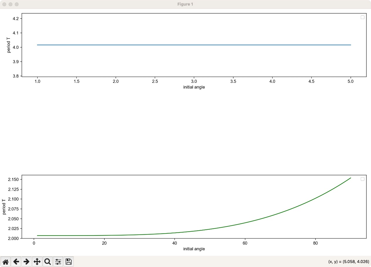
Figure 3: The relationship between T and very small initial angle

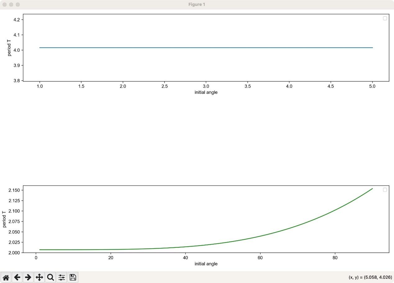
Figure 4: The relationship between T and very initial angle in whole range

In Figure 3 and Figure 4, the horizontal coordinate represents the angle in the degree system, the angle value is 0 in the direction perpendicular to the horizontal line, the positive angle value to the right of the vertical line is the initial angle value, and the vertical coordinate represents the time in seconds

Figure 3 represents the relationship between initial angle and period when pendulum starts with small angle. The study indicates that there is no relationship between period and the initial angle when pendulum starts with very small initial angle.

Figure 4 represents the relationship between initial angle and period when pendulum starts with big angle. It indicates that there exists a completely positive relationship between period T and the initial angle of pendulum.

5. Double pendulum system

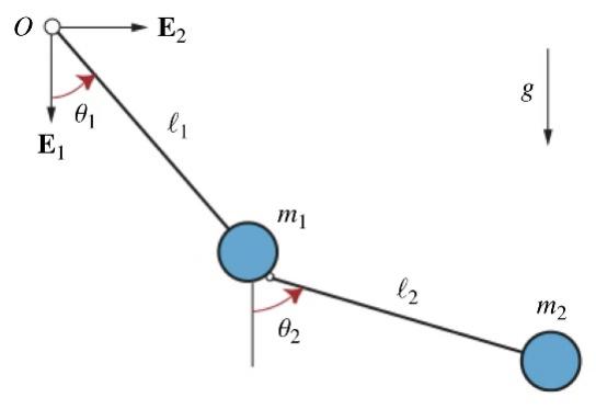
Figure 5: The physical setting of the double pendulum

From a historical perspective, Newton’s Second Law is fundamental [7]. Also, it is widely recognized that physical systems can be effectively characterized by their Lagrangian, and the Lagrangian function enables the derivation of second-order differential equations governing the dynamics of such systems [8]. So next, the study will explain the Lagrangian equation of motion for a 2D double spring-pendulum [9].

Figure 5 is the physical diagram of the double pendulum system. When the radius of the two balls is ignored, \( {l_{1}} \) is the pendulum length of the motion of ball 1, \( {l_{2}} \) is the pendulum length of the motion of ball 2, and \( {θ_{1}} \) and \( {θ_{2}} \) are the initial angles of the motion of the two balls. From the above definition, the study lists expressions for the positions of the two balls.

Assume 1. Point masses 2. Massless rigid rods 3. Gravity is present, with a bunch of equations [7],

\( {x_{1}}={l_{1}}sin{{θ_{1}}}\ \ \ (66) \)

\( {y_{1}}={-l_{1}}cos{θ_{1}}\ \ \ （67） \)

\( {x_{2}}={l_{1}}sin{θ_{1}}+{l_{2}}sin{θ_{2}}\ \ \ （68） \)

\( {y_{2}}=-{l_{1}}cos{θ_{1}}-{l_{2}}cos{θ_{2}}\ \ \ （69） \)

\( \frac{d{x_{1}}}{dt}={ω_{1}}{l_{1}}cos{{θ_{1}}}\ \ \ (70) \)

\( \frac{d{y_{1}}}{dt}={ω_{1}}{l_{1}}sin{{θ_{1}}}\ \ \ (71) \)

\( \frac{d{x_{2}}}{dt}={ω_{1}}{l_{1}}cos{{θ_{1}}}+{ω_{2}}{l_{2}}cos{{θ_{2}}}\ \ \ (72) \)

\( \frac{d{y_{2}}}{dt}={ω_{1}}{l_{1}}sin{θ_{1}}+{ω_{2}}{l_{2}}sin{θ_{2}}\ \ \ （73） \)

And the research gets the equation which \( V \) represents the potential energy of the system [10],

\( V={m_{1}}g{y_{1}}+{m_{2}}g{y_{2}}.\ \ \ (74) \)

Substitute Eq. 67 and Eq. 69 into Eq. 74, it gets,

\( V=-({m_{1}}+{m_{2}})g{l_{1}}cos{{θ_{1}}}-{m_{2}}g{l_{2}}cos{{θ_{2}}}.\ \ \ (75) \)

Then, there is an equation which \( T \) represents the kinetic energy of the system [10],

\( T=\frac{1}{2}{m_{1}}{{v_{1}}^{2}}+\frac{1}{2}{m_{2}}{{v_{2}}^{2}} \)

\( =\frac{1}{2}{m_{1}}({\frac{d{x_{1}}}{dt}^{2}}+{\frac{d{y_{1}}}{dt}^{2}})+\frac{1}{2}{m_{1}}({\frac{d{x_{2}}}{dt}^{2}}+{\frac{d{y_{2}}}{dt}^{2}})\ \ \ (76) \)

Substitute Eq. 71, Eq. 72, Eq. 73 and Eq. 74 into Eq. 76, this study gets,

\( T=\frac{1}{2}{m_{1}}{{ω_{1}}^{2}}+\frac{1}{2}{m_{2}}({{l_{1}}^{2}}{{ω_{1}}^{2}}+{{l_{2}}^{2}}{{θ_{2}}^{2}}+2{l_{1}}{l_{2}}{ω_{1}}{ω_{2}}cos{({θ_{1}}-{θ_{2}})})\ \ \ (77) \)

So, the Lagrangian [7],

\( L=T-V \)

\( =\frac{1}{2}{m_{1}}{{ω_{1}}^{2}}+\frac{1}{2}{m_{2}}({{l_{1}}^{2}}{{ω_{1}}^{2}}+{{l_{2}}^{2}}{{θ_{2}}^{2}}+2{l_{1}}{l_{2}}{ω_{1}}{ω_{2}}cos{({θ_{1}}-{θ_{2}})}) \)

\( +({m_{1}}+{m_{2}})g{l_{1}}cos{{θ_{1}}}+{m_{2}}g{l_{2}}cos{{θ_{2}}}\ \ \ (78) \)

Using the Lagrange’s Equation [11-13],

\( \frac{d}{dt}(\frac{dL}{d{ω_{j}}})-\frac{dL}{d{θ_{j}}}=0 (j=1,2,3,……,n)\ \ \ (79) \)

The study can get the final solution,

\( \begin{array}{c} ({m_{1}}+{m_{2}}){l_{1}}{α_{1}}+{m_{2}}{l_{2}}{α_{2}}cos{({θ_{1}}-{θ_{2}})} \\ +{m_{2}}{l_{2}}{{ω_{2}}^{2}}sin{({θ_{1}}-{θ_{2}})}+({m_{1}}+{m_{2}})gsin{{θ_{1}}}=0.\ \ \ (80) \end{array} \)

Then,

\( {m_{2}}{l_{2}}{α_{2}}+{m_{2}}{l_{1}}{α_{2}}cos{({θ_{1}}-{θ_{2}})}-{m_{2}}{l_{1}}{{ω_{2}}^{2}}sin{({θ_{1}}-{θ_{2}})}+{m_{2}}gsin{{θ_{2}}}=0\ \ \ (81) \)

To solve Eq. 80[7] and Eq. 81[7], first, it uses the small angle approximation to simplify the two equations, let,

\( u=\frac{{m_{1}}}{{m_{2}}}+1\ \ \ (82) \)

\( sin{({θ_{1}}-{θ_{2}})}≈{θ_{1}}-{θ_{2}}\ \ \ (83) \)

\( cos{({θ_{1}}-{θ_{2}})}≈cos{0}=1\ \ \ (84) \)

Then,

\( {α_{1}}=\frac{g{θ_{2}}-ug{θ_{1}}}{{l_{1}}(u-1)}\ \ \ (85) \)

\( {α_{2}}=\frac{ug{θ_{1}}-ug{θ_{2}}}{{l_{2}}(u-1)}\ \ \ (86) \)

Note that Eq. 85[14] and Eq. 86[14] are applicable only when two balls both start with small angles.

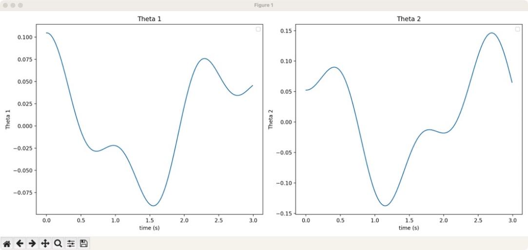
Figure 6: The relationship between theta 1 and time

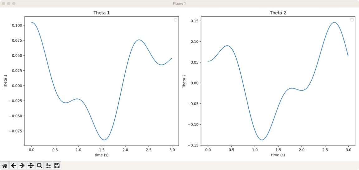
Figure 7: The relationship between theta 2 and time

Figure 6 and Figure 7 represent the relationship between the two angles in the double pendulum over time, so that the one perpendicular to the horizontal line represents the 0-angle value, and the right side of the vertical line represents the positive Angle value and the left side represents the negative angle value. angles are expressed in the degree system.

Figure 6 and Figure 7 are plotted based on Eq. 85 and Eq. 86.

From Figure 6, it indicates that within three seconds, the image of Theta 1 has five inflection points of the change trend, where the maximum value is the initial value, while the minimum value is negative, which appears at about 1.6 seconds. From Figure 7, it indicates that the image of Theta 2 also has five inflection points of the change trend, reaching the maximum value at about 2.7 seconds and the minimum value at about 1.2 seconds.

6. Comparison and result

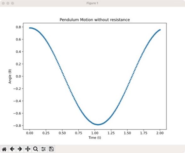
Figure 8: The numerical solution of pendulum without resistance

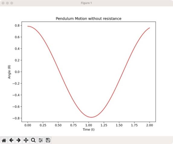
Figure 9: The analytical solution of pendulum without resistance

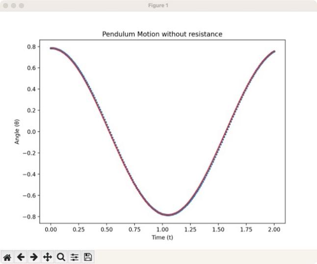
Figure 10: The comparison between analytical solution and numerical solution of pendulum without resistance

Figure 8 is the image of the numerical solution of the pendulum, and Figure 9 is the image of the analytical solution of the pendulum. Figure 8 and Figure 9 are plotted under the same initial conditions, so this study compares them in one single plot—Figure 10.

In Figure 10, the horizontal coordinate represents the angle in the radian system, the angle value is 0 in the direction perpendicular to the horizontal line, the positive angle value to the right of the vertical line is the initial angle value, and the vertical coordinate represents the time in seconds.

In order to better compare the image of the numerical solution and the image of the analytical solution of a simple pendulum without resistance, the research plots them in the same figure, with the solid line representing the analytical solution and the dotted line representing the numerical solution. Because both the numerical equation and analytical solution are built when there is no resistance on the simple pendulum, it doesn’t need to approximate much when building the numerical equation, so their images almost overlap over the whole domain. Obviously, Figure 8 represents a good approximation.

Then, look into the images of the numerical solution and analytical solution of a simple pendulum with resistance. Because both the numerical equation and analytical solution are built when there is resistance on the simple pendulum, the value of the damping coefficient of air friction may have an effect on the accuracy of the approximation.

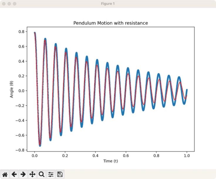
Figure 11: The comparison between analytical solution and numerical solution of pendulum with resistance

In Figure 11, the horizontal coordinate represents the angle in the radian system, the angle value is 0 in the direction perpendicular to the horizontal line, the positive angle value to the right of the vertical line is the initial angle value, and the vertical coordinate represents the time in seconds.

7. Conclusion

This study looked at a simple pendulum moves under different initial conditions. By creating a model of harmonic motion and using Newton's laws, this study found the differential equations that describe the pendulum's motion and analyzed them. The analytical method solved the equations to give a clear formula showing how the pendulum's angle changes over time. This strategy highlighted the pendulum's periodic character and the impact of its beginning circumstances. The numerical technique gave some practical answers and demonstrated its applicability in more complicated scenarios. The study also accounted for air resistance by adding a factor to the equations. This showed how air resistance changes the pendulum's amplitude and period. In summary, both methods gave valuable insights into the pendulum's behavior. This study also analyzed the motion of a double pendulum using Lagrange's equation. The analytical solution offers a more succinct description, even though the numerical technique may be modified to accommodate ever more complicated circumstances. Together, the study improves the understanding of pendulum dynamics and paves the way for future studies on more complex systems.

Authors’ contributions

Xinyue Luo wrote python code and drew numerical and analytical python images for each stage of the paper. She is responsible for the motion equation of the relationship between initial angle and period and the research about Double Pendulum System. She is also responsible for the comparison and results in part.

Xu Ruolin derived and proved the numerical and analytical functions of simple pendulums with and without resistance. She was responsible for the derivation of the equations of motion and the small angular period of simple pendulums with and without air resistance.

Yanxin Jiang provided help in data collection, prepared the introduction and end of the presentation, summarized data and formulas, and took charge of PPT production. She is responsible for the abstract, introduction and conclusion of the paper.

Acknowledgment

Xinyue Luo, Ruolin Xu and Yanxin Jiang contributed equally to this work and should be considered co-first authors.

References

[1]. Daniel, R. Acoustics and Vibration Animations <http: // www.acs.psu.Edu/ drussell/ Demos/ Pendulum/ Pendula.html>.
[2]. Boston University Physics Department. Torque and rotational inertia Physics lecture demonstrations at Boston University. <https://physics.bu.edu/˜duffy/py105/Torque.html>.
[3]. Graber-Mitchell, N. (2018) Finding the period of a simple pendulum. arXiv: Classical Physics.
[4]. Austin Christian. Math 31A Discussion Session 2016. <http://www.math.ucla.edu/˜archristian/ teaching/31a-w16/week-2.pdf>.
[5]. Tseng, Z. S. Second Order Linear Differential Equations 2016. <http: // www.math.psu.edu/ tseng/ class/ Math251/ Notes-2nd%20order%20ODE%20pt1.pdf>.
[6]. Mohazzabi, P., & Shankar, S. P. (2016). Damping of a simple pendulum due to drag on its string. Journal of Applied Mathematics and Physics, 5(1), 122-130.
[7]. Elbori, A., & Abdalsmd, L. (2017). Simulation of double pendulum. J. Softw. Eng. Simul, 3(7), 1-13.
[8]. Baleanu D, Asad, JH, Petras I. 2015. Numerical solution of the fractional Euler Lagrange’s equations of a thin elastic model. Nonlinear Dynamics 81: 97-102. https://doi.org/10.1007/s11071-015-1975-7
[9]. Nenuwe, N. O. (2019). Application of Lagrange equations to 2D double spring-pendulum in generalized coordinates. Ruhuna Journal of Science, 10(2).
[10]. Rafat, M. Z., Wheatland, M. S., & Bedding, T. R. (2009). Dynamics of a double pendulum with distributed mass. American Journal of Physics, 77(3), 216-223.
[11]. Martin C, Salomonson P. 2009. An introduction to analytical mechanics, 4th edn. Goteborg Sweden 1-62 pp.
[12]. Murray RS. 1967. Theoretical mechanics, Schaum’s outlines, Mcgraw-Hill 299 – 301 pp.
[13]. Goldstein H, Poole C, Safko J. 2000. Classical mechanics, 3rd edn. Addison Wesley, New York, 5-69.
[14]. Shinbrot, T., Grebogi, C., Wisdom, J., & Yorke, J. A. (1992). Chaos in a double pendulum. American [4]cs.bu.edu/˜duffy/py105/Torque.html>.
Cite this article
Luo,X.;Xu,R.;Jiang,Y. (2025). Simulation of Simple Pendulums with Different Stages. Theoretical and Natural Science,107,25-40.
Data availability
The datasets used and/or analyzed during the current study will be available from the authors upon reasonable request.
Disclaimer/Publisher's Note
The statements, opinions and data contained in all publications are solely those of the individual author(s) and contributor(s) and not of EWA Publishing and/or the editor(s). EWA Publishing and/or the editor(s) disclaim responsibility for any injury to people or property resulting from any ideas, methods, instructions or products referred to in the content.
About volume
Volume title: Proceedings of the 4th International Conference on Computing Innovation and Applied Physics
© 2024 by the author(s). Licensee EWA Publishing, Oxford, UK. This article is an open access article distributed under the terms and
conditions of the Creative Commons Attribution (CC BY) license. Authors who
publish this series agree to the following terms:
1. Authors retain copyright and grant the series right of first publication with the work simultaneously licensed under a Creative Commons
Attribution License that allows others to share the work with an acknowledgment of the work's authorship and initial publication in this
series.
2. Authors are able to enter into separate, additional contractual arrangements for the non-exclusive distribution of the series's published
version of the work (e.g., post it to an institutional repository or publish it in a book), with an acknowledgment of its initial
publication in this series.
3. Authors are permitted and encouraged to post their work online (e.g., in institutional repositories or on their website) prior to and
during the submission process, as it can lead to productive exchanges, as well as earlier and greater citation of published work (See
Open access policy for details).