1. Introduction

A device in which a small object is suspended from one end of an in inelastic slight rope is defined as a pendulum. When a pendulum is released, the restoring force combined the mass of it so it can oscillate about the equilibrium position. Single pendulum is one of the most basic physical phenomena for observing resonant oscillation motion.

Besides, with the development of the artificial intelligent, computer can make sketching and drawing trajectory of objects easier. Using programming language and graphics software, complex physical models and motion processes can be showed directly, thus it can show the non-linear motion of pendulum easily. As a general programming language, Python is widely used and learned because of its free and open source, flexible and easy to learn, powerful and other advantages.

In this work, we starting from the perspective of Newton's second law, using mathematical methods such as Taylor expansion to solve the numerical solution and analytical solution in the case of changing different variables, and using Python to draw pictures comparison, so as to carry out a detailed study of the motion of a simple pendulum in general.

2. Theoretical deduction

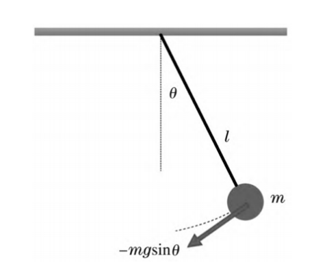
Figure 1: Elements in pendulum motion[1]

As shown in figure 1, a simple pendulum system consists of a pendulum ball with mass m and a thin rod with negligible mass. The pendulum length l, and angle θ at time t. For the convenience of calculation, we set the length of the string( \( l \) ) is \( 1cm \) and initial velocity equals to 0 rad/s, and acceleration of gravity \( g \) is \( 9.8\frac{m}{{s^{2}}}. \)

A right-angle coordinate system should be set up along the direction of the string pulls, after which the force of gravity can be decomposed. The force provided by the string and the force of the y-axis component of gravity can be contracted. Let us now consider the scenario in which the experimenter manually pulls the ball to the right, as illustrated in the figure. Given that the ball is in decelerated motion, the displacements and accelerations are in opposite directions, consequently, the force towards the left half-axis of the x-axis in the diagram is negative \( mgsinθ \) [1].

Tangential acceleration of the ball can be expressed by[2]

\( {α_{T}}=l\frac{{d^{2}}θ}{d{t^{2}}} \) (1)

drag force

\( {F_{T}}=-γv=-γl\frac{dθ}{dt} \) (2)

according to Newton’s Second Law

\( -mgsinθ+γl\frac{dθ}{dt}=ml\frac{{d^{2}}θ}{d{t^{2}}} \) (3)

Equation (3) describes the dynamic equilibrium of a pendulum considering damping effects. \( -mgsinθ+γl\frac{dθ}{dt} \) represent the total external forces acting on the system, while \( ml\frac{{d^{2}}θ}{d{t^{2}}} \) represents how the motion state of the pendulum changes over time. When the two parts are equal, the system reaches dynamic equilibrium.

3. Numerical solutions and graphs

3.1. Simple harmonic motion

To prove the equation of the free oscillation of a simple pendulum, we can use the Taylor expansion to approximate the solution[3].

First, we expand the Angle \( θ \) to the second order term. The general form of Taylor expansion is as follows:

\( f(x)=f(a){+f^{ \prime }}(a)(x-a)+\frac{1}{2!}{f^{ \prime \prime }}(a){(x-a)^{2}}+…+\frac{{f^{n}}(a)}{n!}{(X-a)^{n}}+{R_{n}}(x) \) (4)

In this case, we only need to expand to the quadratic term. For the Angle \( θ \) , we can choose to expand with \( θ=0 \) as the center. According to Taylor's definition of expansion, we have:

\( θ=θ(0)t{+θ^{ \prime }}(0)t+\frac{1}{2}{θ^{ \prime \prime }}(0){(t)^{2}} \) (5)

Where \( θ(0) \) represents the initial angle, \( θ \prime (0) \) represents the initial angular velocity, and \( θ \prime (0) \) represents the initial angular acceleration.

Since we are concerned with the equation of motion in the case of free vibration, assume that the initial angle is 0, that is, \( θ(0)=0 \) , and the initial angular velocity is 0, that is \( θ \prime (0)=0 \) . Therefore, the equation (5) can be simplified to:

\( \frac{{d^{2}}θ}{dt}=θ \prime \prime (0) \) (6)

Now let's consider the equation of motion of a simple pendulum. According to the motion law of a simple pendulum, when the swing Angle is small, the \( sinθ \) can be approximated to \( θ \) . Therefore, we can approximate \( θ \prime \prime (0) \) as \( -\frac{g}{l}θ(0) \) . Substituting this approximation into the equation (6) gives us:

\( \frac{{d^{2}}θ}{d{t^{2}}}=-\frac{g}{l}θ(0) \) (7)

\( \frac{{d^{2}}θ}{d{t^{2}}}=-\frac{g}{l}sinθ \) (8)[4]

The equation (8) is the approximate formula of motion for the free vibration of a simple pendulum. Note that the equation (8) holds if the swing angle is small, that is, if \( θ \) is close enough to 0.

In summary, by Taylor expansion and approximate solution, we prove that the equation of free vibration of a simple pendulum is:

\( \frac{{d^{2}}θ}{d{t^{2}}}=-\frac{g}{l}θ \) (9)

From the equation (9), it can be seen that under the small angle approximation, the equation is a simple harmonic motion equation. This means that the pendulum undergoes simple harmonic motion, oscillating back and forth around its equilibrium position with a fixed period and amplitude.

3.2. Regular pendulum motion

Without considering damping and torque driving, the torque on the pendulum is[5]:

\( M=-mgsinθl \) (10)

According to the law of rotation, we get

\( M=-mgsinθl=m{l^{2}}\frac{{d^{2}}θ}{d{t^{2}}} \) (11)

The equation of free vibration of a simple pendulum is obtained as[6,7]

\( \frac{{d^{2}}θ}{d{t^{2}}}=-\frac{g}{l}θ \) (12)

It can be seen that the free vibration equation of a simple pendulum can be derived from the above two methods. And the initial conditions of this equation can be expressed as:

\( \frac{dθ(t=0)}{dt}=0 \) (13)

We can also express the equation (13) in another form. We typically use discretization methods to convert the differential equations in the time domain into difference equations.

\( \frac{dθ}{dt}≈\frac{{θ^{i}}-{θ^{i-1}}}{Δt} \) (14)

\( \frac{{d^{2}}θ}{dt}≈\frac{1}{Δt}(\frac{{θ^{i+1}}-{θ^{i}}}{Δt}-\frac{{θ^{i}}-{θ^{i-1}}}{Δt})=\frac{{θ^{i+1}}-2{θ^{i}}+{θ^{i-1}}}{Δ{t^{2}}} \) (15)

\( \frac{{θ^{i+1}}-2{θ^{i}}+{θ^{i-1}}}{Δ{t^{2}}}=\frac{-g}{L}sin{θ^{i}} \) (16)

The equation (16) indicates that at each time step (i), the change in angular displacement is proportional to the sine of the current angle, thereby illustrating the dynamic behavior of the pendulum during small-angle oscillations.

Moreover, the graph of the numerical solution is presented below for illustrative purposes.

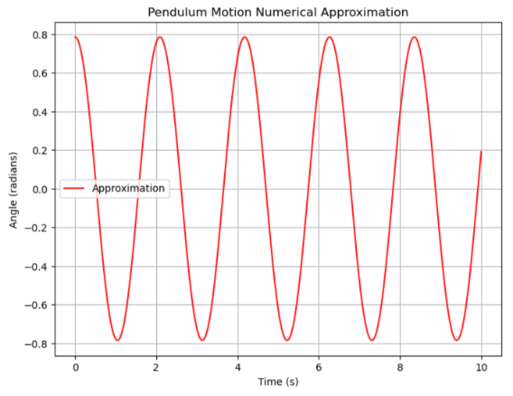
Figure 2: Numerical approximation of pendulum motion[8]

From figure 2 we can know that, in the absence of damping or external forces, the total mechanical energy of the pendulum should be conserved, which is reflected in the consistent maximum angle (amplitude) in each period shown in the graph. That is, the amplitude of each peak and trough is equal. Figure 2 displayed a periodic curve. A pendulum, under ideal conditions without damping forces, exhibits periodic motion, with its angle varying over time in the form of a sine or cosine curve. This indicates that the pendulum is a periodic system, with its period (T) being influenced by the pendulum length (l) and gravitational acceleration (g).

3.3. Analytical solutions and graphs

In addition to the numerical solution, which includes the approximation, we are now attempting to identify the analytical solution[9]. This entails reformulating the problem in a well-understood form and calculating the exact solution. We have:

\( \frac{{d^{2}}θ}{d{t^{2}}}+\frac{g}{l}θ=0 \) (17)

This is a second order linear homogeneous differential equation with constant coefficients.

To understand the equation (17), we can first find its characteristic equation. Assuming the solution is of the form \( θ(t)={e^{rt}} \) , plug it into the differential equation:

\( {r^{2}}{e^{rt}}+\frac{g}{l}{e^{rt}}=0 \) (18)

By solving the second order linear homogeneous differential equation with the eigen equation method, we derive the solution of the simple pendulum under the small angle approximation:

\( θ(t)={c_{1}}cos\sqrt[]{\frac{g}{l}}+{c_{2}}sin\sqrt[]{\frac{g}{l}} \) (19)

Where \( {c_{1}} \) and \( {c_{2}} \) are constants determined by the initial conditions.

The structure of equation (19) is similar to the solution of a simple harmonic oscillator, which contains sine and cosine components.

\( \sqrt[]{\frac{g}{l}} \) is the angular frequency \( ω \) of the system. For a simple pendulum, the angular frequency \( ω=\sqrt[]{\frac{g}{l}} \) . \( cos⁡(ωt) \) and \( sin⁡(ωt)⁡ \) are sine and cosine functions that describe simple harmonic motion. The final formula of analytical solution can be understood as:

\( θ={c_{1}}cos(ωt)+{c_{2}}sin{(ωt)} \) (20)

Equation (20) shows that the change of angle θ with time t is a simple harmonic motion. The values of \( {c_{1}} \) and \( {c_{2}} \) depend on the initial conditions of the system at t=0.

As a result, the graph of analytical solution is shown below.

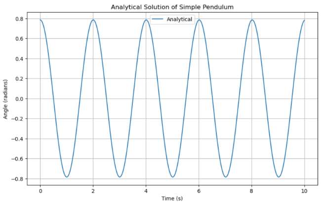
Figure 3: Analytical solution of pendulum motion

As expected, the curve of figure 3 exhibits a very similar trend to the curve of figure 2. Next we will proceed with a comparative analysis of the two figures.

3.4. Comparison of numerical and analytical solutions

Following an investigation of the numerical and analytical solutions, the new problem is to ascertain the difference between the two solutions. The objective here is to identify the relationship between error and time and to consider why the numerical solution is not as exact as the analytical one.

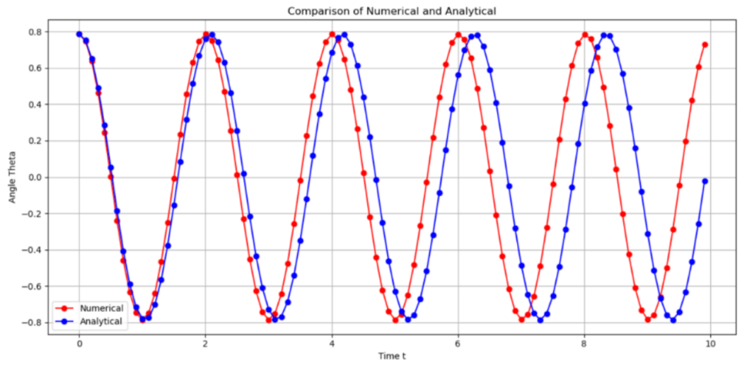
Figure 4: Difference between analytical and numerical solutions

Figure 4 depicts a comparison between the numerical and analytical solutions. The blue line represents the analytical method, while the red line illustrates the numerical solution. It is evident that the discrepancy between the two waves is progressively increasing. However, it remains unclear whether the relationship is linear, exponential, or otherwise. It is therefore necessary to calculate the value of each gap and plot a graph in order to directly demonstrate the relationship.

\( Error=Analytical-Numerical \)

The equation above is employed to ascertain the disparity between the numerical and analytical solutions at varying points in time.

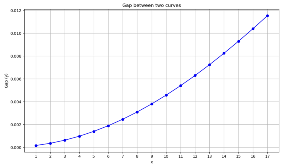
Figure 5: Relationship between gap and time

From figure 5, at the beginning, the gap is nearly zero, which signifies that the two waves are approximately superimposed, consequently, the value of the difference is 0.0, evidenced in the data collection as index 0 on the left. The final stage of the process is to collect all the data and create a graph to illustrate the discrepancy between the two waves. Figure 5 illustrates an exponential growth trend, indicating that the rate of change in the gap will increase over time. As a result, the longer the unit period, the greater the degree of inaccuracy in the numerical solution.

3.5. Change in variables

In this section, the objective is to utilize the control variable method to modify specific elements and subsequently analyze the resulting alterations in the graphs. Consequently, it is possible to ascertain which elements exert an influence on the position of the mass suspended at the end of the string.

3.5.1. Initial angle

The first variable changed is initial angle which is the theta in the equation. First, we set the 45º to be the default value which is shown as black and pick other degree to compare with the default value. The following graphs illustrate three different comparisons between the default value and correspondently 30º, 60º and 75º.

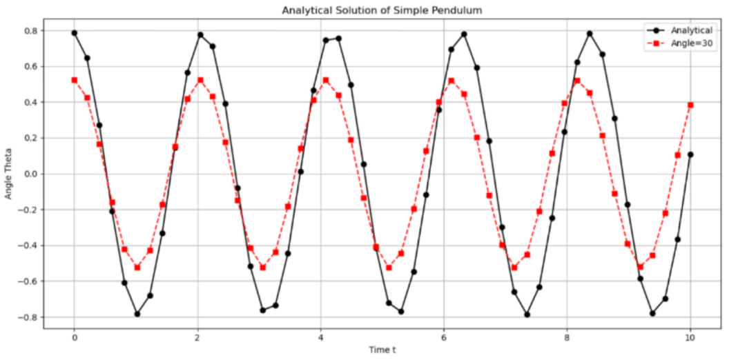
Figure 6: Analytical solution of pendulum (initial angle=30)

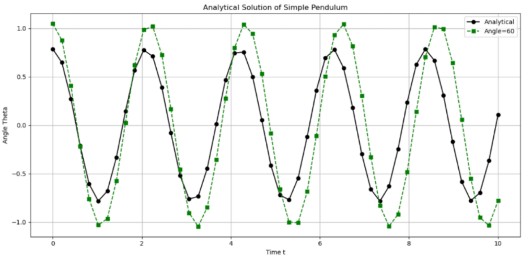
Figure 7: Analytical solution of pendulum (initial angle=60)

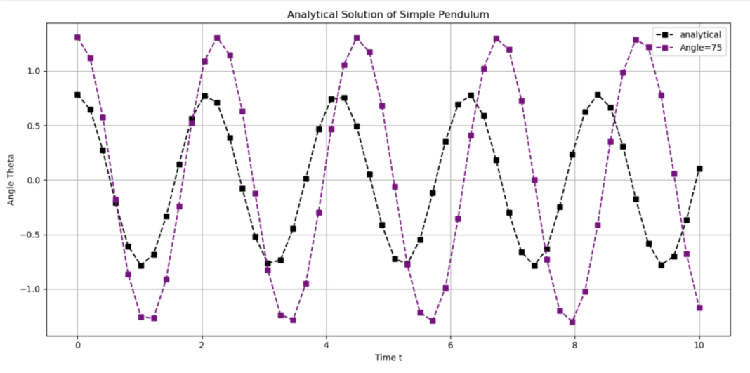
Figure 8: Analytical solution of pendulum (initial angle=75)

From figure 6-8, it is evident that the peak of the red wave (Figure 6) is lower than that of the default graph. However, the second graph indicates that the peak of the green wave (Figure 7) is higher. Furthermore, the peak of the purple wave (Figure 8) is considerably higher. Considering these observations, it can be posited that the initial angle exerts an influence on the amplitude of the wave, which represents the maximum angle that the ball can reach. Also, the distances between two adjacent peak, the unit time periods, are different in each graph, indicating that the initial angle has impact on unit period. To facilitate a more comprehensive analysis, the three graphs have now been superimposed in the same coordination system.

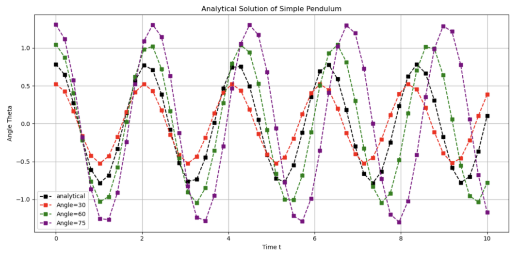
Figure 9: Comparison of different angle with default value

As shown in figure 9, as the increasing in initial angle, the motion period of the pendulum also increases, and the amplitude of the change in pendulum angle increases.

The initial stage of the investigation entails establishing the relationship between the initial angle and the maximum angle that the ball can reach. Figure 10, created by Python programming language, illustrates how max angle depends on initial angle. Obviously, the relationship is linear related and positive proportional.

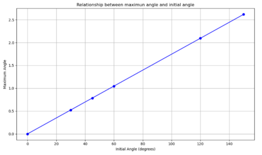
Figure 10: Relationship between maximum angle and initial angle

Moreover, it is anticipated that a discussion will be held regarding the correlation between the initial angle and the unit period.

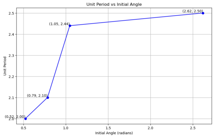
Figure 11: Relationship between unit period and initial angle

As can be observed in the figure 11, the relationship is not linear; however, it is evident that the trend is increasing based on the plotted points. Therefore, the larger the initial angle, the longer the unit period.

3.5.2. Length of string

The second variable that undergoes a change is the length of the string, which is represented by the letter \( l \) . Additionally, the \( 1m \) value was designated as the default, indicated in black, and the remaining lengths were selected for comparison with the default value. The following graphs illustrate four distinct comparisons between the default value and the corresponding values of \( 0.5m \) , \( 5m \) , \( 10m \) and \( 50m \) .

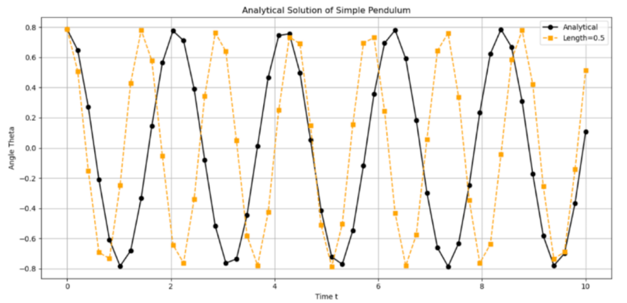
Figure 12: Analytical solution of pendulum (length =0.5)

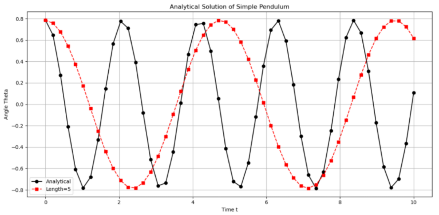
Figure 13: Analytical solution of pendulum (length =5)

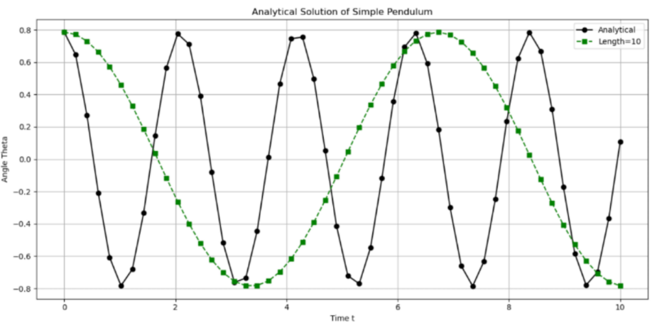
Figure 14: Analytical solution of pendulum (length =10)

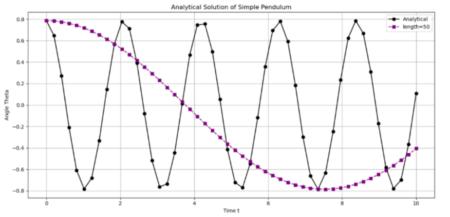
Figure 15: Analytical solution of pendulum (length =50)

From the figure 12-15, it can be observed that as the length of the wave increases, the wave appears to be stretched. Consequently, the unit period is dependent on the value of length. In the absence of any frictional forces and with the initial conditions held constant, the amplitude which represents the max angle the ball can reach remains unaltered. Similarly, to produce a much clearer analysis, the four graphs have now been superimposed in the same coordination system shown below.

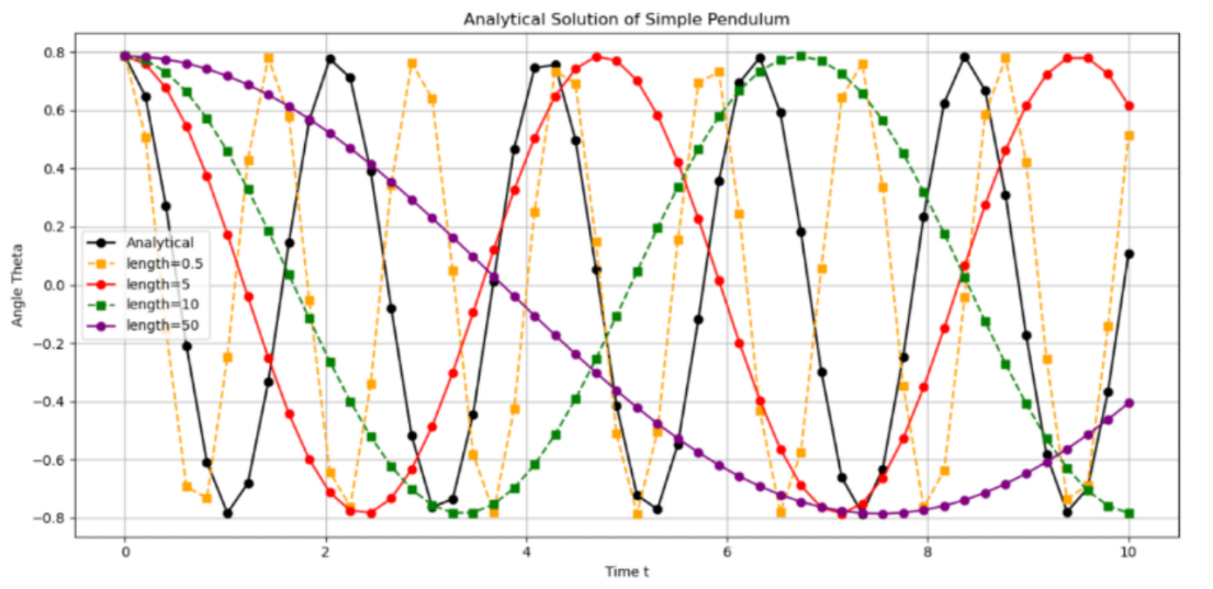
Figure 16: Comparison of different length with default value

A cursory examination of the figure 16 reveals that the wave in question is elongated from the yellow to the purple segment. In particular, the distance between two adjacent peaks can be calculated to obtain the unit period under each condition. To gain a more comprehensive understanding, a best-fit line has been drawn using the five points.

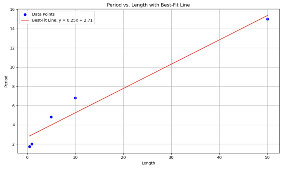
Figure 17: Relationship between period and length

According to figure 17, although not linear related, it is evident that the trend displays an increase as the length increases.

3.5.3. Initial velocity

The final section concerns the alteration of the initial velocity while maintaining the initial angle and length of string consistent with the preceding assumption. The initial velocity is modified from 0 radian per second, which represents the default value, to 5 radian per second, and a graph is generated using the Python programming language.

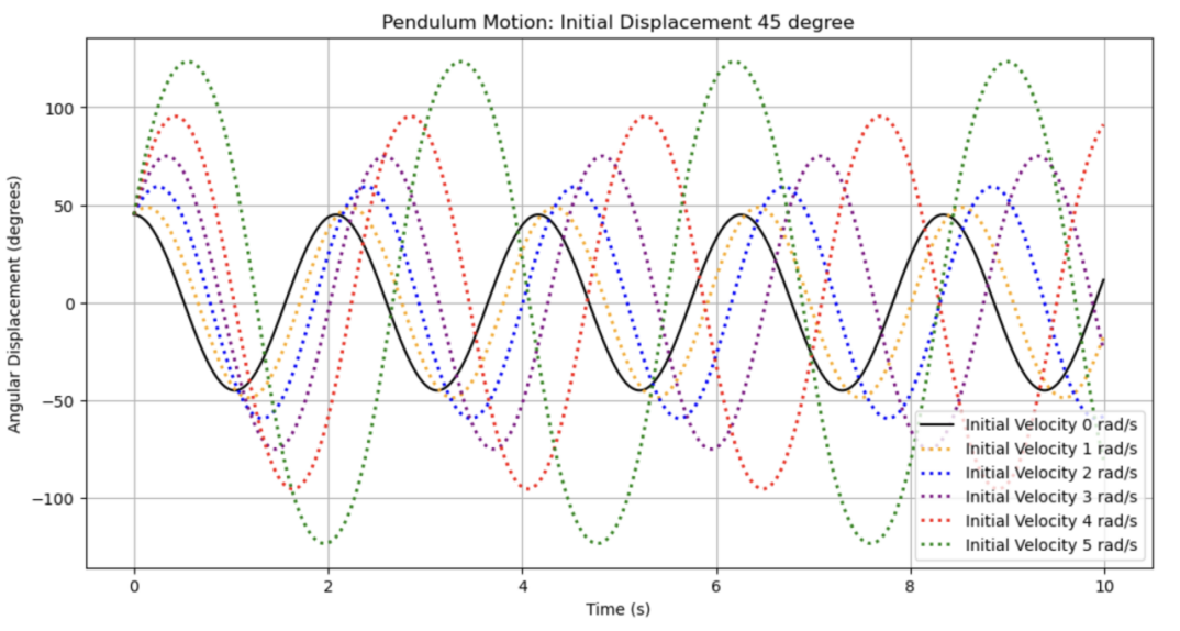
Figure 18: Comparison of various initial velocity with default value

From an examination of the figure 18, it can be discerned that the wave is stretched in both the horizontal and vertical dimensions, in accordance with the parameters of the default graph. It can thus be inferred that there is a relationship between the initial velocity, the maximum angle and the unit period.

The objective of this investigation is to ascertain the relationship between the unit period and the initial velocity.

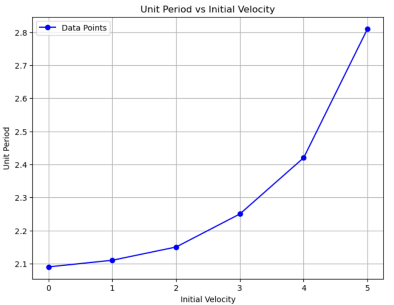
Figure 19: Relationship between unit period and initial velocity

From the figure 19, there is an exponential relationship between the two variables. It can therefore be concluded that, in addition to the inverse relationship between initial velocity and unit period, there is also an inverse relationship between the rate of change of unit period and initial velocity.

Subsequently, focusing on how the max angle depends on the initial velocity in figure 20, it can be demonstrated that the relationship between these two variables is also increasing.

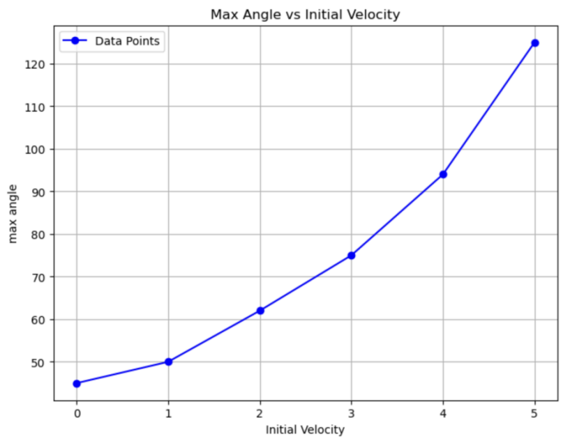
Figure 20: Relationship between max angle and initial velocity

4. With drag force

4.1. Analytical solutions

In the case of small pendulum angles, assume the mass of the pendulum bob is \( m \) =1kg, and the length of the pendulum string is \( l \) =1m. The tangential acceleration of the pendulum bob is given by:

\( a=l\frac{{d^{2}}θ}{d{t^{2}}} \) (21)

During its motion, the simple pendulum is subject to the forces of gravity, drag, and tension from the string. The drag force primarily comes from air resistance, which is proportional to the velocity when the speed is not too high[10,11]. The drag force acts in the direction tangent to the motion as follows:

\( F=-γv=-γl\frac{dθ}{dt} \) (22)

where γ is the proportionality constant in the tangential direction. According to Newton's second law, we obtain[2]

\( -mgsinθ+γl\frac{dθ}{dt}=ml\frac{{d^{2}}θ}{d{t^{2}}} \) (23)

The equation (23) is a second-order linear differential equation describing the motion of pendulum[12]. We rearrange the equation into standard form, which is the auxiliary equation then set \( \frac{dθ}{dt} \) is \( r \) so the original equation can be converted into

\( ml{r^{2}}-lγr+mgsinθ=0 \) (24)

In this case we can use quadratic equation formula to get the equation of \( r \) .

\( r=\frac{lγ±\sqrt[]{4{m^{2}}lgsinθ-{l^{2}}{γ^{2}}}i}{2ml} \) (25)

In theory, there are three situations for the solution of equation (25) (when \( {l^{2}}{γ^{2}}-4{m^{2}}lgsinθ \) is greater than zero, equal to zero and less than zero), but due to the the actual situation analysis, the first two cases must be dropped, so we can get

\( θ={e^{\frac{lγθ}{2ml}}}({c_{1}}cos{\frac{\sqrt[]{4{m^{2}}lgsinθ-{l^{2{γ^{2}}}}}}{2ml}θ}+{c_{2}}sin{\frac{\sqrt[]{4{m^{2}}lgsinθ-{l^{2}}{γ^{2}}}}{2ml}θ}) \) (26)

Now we have the expression of \( θ \) . Where \( {c_{1}} \) and \( {c_{2}} \) are arbitrary constants.

Then we use Python to draw the graph of it. In figure 21, it illustrates how the damped pendulum changes over time, showing the process of energy loss due to the effect of damping.

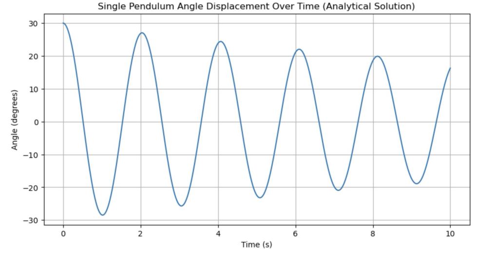
Figure 21: Analytical solution for pendulum motion with drag

4.2. Numerical solutions

We assume \( {θ_{1}}=θ \) and \( {θ_{2}}=\frac{dθ}{dt} \) , so the original equation can be rearranged as follows:

\( \frac{d{θ_{1}}}{dt}={θ_{2}} \) (27)

\( \frac{d{θ_{2}}}{dt}=-\frac{g}{l}sin{θ_{1}}+\frac{γ}{m}{θ_{2}} \) (28)

We used the integration method to solve the above linear differential equation. So equation 28 can be expressed as:

\( \frac{d{θ_{2}}}{dt}+\frac{γ}{m}{θ_{2}}=-\frac{g}{l}sin{θ_{1}} \) (29)

Assuming we know the change in \( {θ_{1}} \) , we can define an integrating factor:

\( {e^{∫(\frac{γ}{m})dt}}={e^{\frac{γ}{m}t}} \) (30)

By simplifying and solving equation (30), we substitute \( {θ_{1}} \) back into the equation to solve for \( θ \) and \( {θ_{1}} \) , thereby obtaining the numerical solution. Based on this approach, we have derived the numerical solution of the equation, and subsequently, we plotted the graph based on this solution

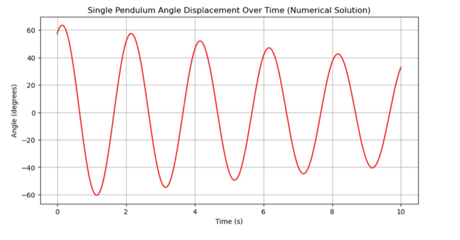
Figure 22: Numerical solution for pendulum motion with drag

From figure 22, it has a similar trend with figure 21; however, there is a certain discrepancy in the time points represented by the peaks of the two figures. Additionally, within the same period, the wave height in figure 22 is significantly greater than that in figure 21.

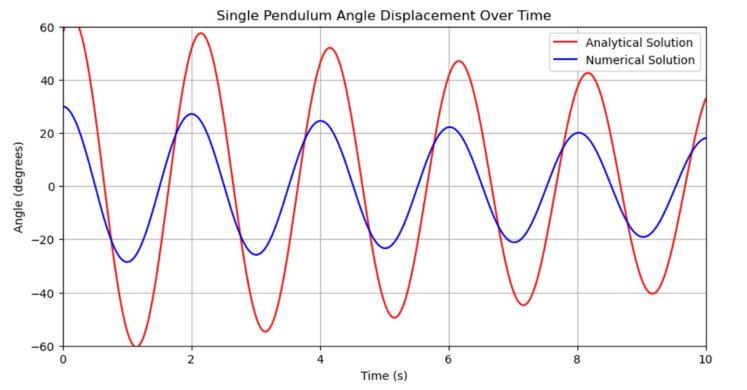
Figure 23: Comparison of analytical and numerical solution

As shown in the figure 23, the error between the analytical solution and the numerical solution gradually decreases over time, which indicates that the adopted mathematical model and assumptions can adequately describe the actual behavior of the pendulum motion.

5. Conclusion

In the study of pendulum motion, a larger initial angle results in both a greater maximum angle and an increased unit period of oscillation. Additionally, as the length of the string increases, the wavelength of the oscillation graph also enlarges, which suggests that, assuming the initial angle remains unchanged and air drag is neglected, the time taken for each swing per period increases with the length of the string. Furthermore, both the initial velocity and the maximum angle exhibit exponential growth concerning the unit period. Lastly, the amplitude of the curve decreases continuously, illustrating that when air drag is considered, both the swing angle and the displacement of the pendulum reduce over time.

Acknowledgement

Zijun Xu and Zhihui Jin contributed equally to this work and should be considered co-first authors.

References

[1]. Wei, X., Yang, C., Shang, M., Wang, X., & Wu, Y. (2024). Study on nonlinear dynamics of a single pendulum based on Python. https://doi.org/10.14139/j.cnki.cn22-1228.2024.03.019.
[2]. Sun, J. (2016). Numerical simulation and analysis of simple pendulum motion. https://doi.org/10.13398/j.cnki.issn1673-260x.2016.24.002
[3]. Wu, J. (2024). Application of Taylor Expansion on Calculating Functions. Highlights in Science, Engineering and Technology, 88, 464–469. https://doi.org/10.54097/28kn1016
[4]. Beléndez A, Arribas E, Márquez A, Ortuño M and Gallego S 2011 Approximate Expressions for The Period of a Simple Pendulum using a Taylor Series Expansion Eur. J. Phys. 32 1303–10
[5]. Coullet, P., Gilli, J. M., Monticelli, M., & Vandenberghe, N. (2005). A damped pendulum forced with a constant torque. American Journal of Physics, 73(12), 1122–1128. https://doi.org/10.1119/1.2074027
[6]. Wenwei,M, Xishun, X, Yuqing, Z. Physics (Seventh Edition), Volume 2[M]. Beijing: Higher Education Press, 2020:21⁃38.
[7]. Yunfeng, G. Matlab to solve the series of theoretical mechanics problems (III) Motion and cycle of simple pendulum and elliptic pendulum [J]. Mechanics and Practice, 2021,43(4) :593⁃598.
[8]. Python Tutorial Release 3.5.1 Guido van Rossum and the Python development team. (2016).
[9]. Chai, C., Feng, F., Wang, G., & Wei, F. (2020). Analytical solution and experimental application of “period” variation of a single pendulum with large swing Angle. https://doi.org/10.19655/j.cnki.1005-4642.2020.03.010
[10]. Quiroga, G. D., & Ospina-Henao, P. A. (2017). Dynamics of damped oscillations: physical pendulum. European Journal of Physics, 38(6), 065005. https://doi.org/10.1088/1361-6404/aa8961
[11]. Yakubu, G., Olejnik, P., & Awrejcewicz, J. (2022). On the Modeling and Simulation of Variable-Length Pendulum Systems: A Review. Archives of Computational Methods in Engineering, 29(4), 2397–2415. https://doi.org/10.1007/s11831-021-09658-8
[12]. Thomson Brooks-Cole copyright 2007.
Cite this article
Xu,Z.;Jin,Z. (2025). Simulation and Analysis of Pendulum Motion System with and Without Drag in the Absence of External Forces. Theoretical and Natural Science,107,83-98.
Data availability
The datasets used and/or analyzed during the current study will be available from the authors upon reasonable request.
Disclaimer/Publisher's Note
The statements, opinions and data contained in all publications are solely those of the individual author(s) and contributor(s) and not of EWA Publishing and/or the editor(s). EWA Publishing and/or the editor(s) disclaim responsibility for any injury to people or property resulting from any ideas, methods, instructions or products referred to in the content.
About volume
Volume title: Proceedings of the 4th International Conference on Computing Innovation and Applied Physics
© 2024 by the author(s). Licensee EWA Publishing, Oxford, UK. This article is an open access article distributed under the terms and
conditions of the Creative Commons Attribution (CC BY) license. Authors who
publish this series agree to the following terms:
1. Authors retain copyright and grant the series right of first publication with the work simultaneously licensed under a Creative Commons
Attribution License that allows others to share the work with an acknowledgment of the work's authorship and initial publication in this
series.
2. Authors are able to enter into separate, additional contractual arrangements for the non-exclusive distribution of the series's published
version of the work (e.g., post it to an institutional repository or publish it in a book), with an acknowledgment of its initial
publication in this series.
3. Authors are permitted and encouraged to post their work online (e.g., in institutional repositories or on their website) prior to and
during the submission process, as it can lead to productive exchanges, as well as earlier and greater citation of published work (See
Open access policy for details).