1. Introduction

Linear regression [1], as a cornerstone method in data analysis and predictive tasks, is widely applied in statistical modeling and machine learning. While standard linear regression efficiently extracts linear relationships from simple data through the normal equation [2], its performance faces persistent challenges when dealing with noisy data [3] or high-dimensional features. Based on the least squares method, standard linear regression optimizes the mean squared error [4] for parameter estimation but reveals two critical flaws: First, its lack of regularization constraints struggles to suppress overfitting [5], a limitation particularly evident in datasets with significant noise interference, where initial parameter estimates must align closely with the true data distribution. Second, its reliance on a single analytical solution fails to adapt to the dynamic characteristics of data [6], leading to cascading errors where minor deviations in the training phase can escalate into significant prediction failures during testing.

Recent advances in optimization algorithms, such as Ridge regression [7] and gradient descent [8], have improved model robustness but remain constrained by fixed hyperparameter choices and static loss functions. For instance, the direct solution of standard linear regression overly depends on local data properties, sacrificing global generalization, while traditional regularization methods rely on simplistic penalty configurations. These limitations are particularly detrimental in high-noise predictive tasks, which demand both accurate trend fitting and effective outlier suppression.

To overcome these challenges, we propose a linear regression method based on regularized hyperparameter optimization. This novel strategy introduces two key innovations: a hyperparameter-driven regularization mechanism that dynamically adjusts model complexity via an L2 penalty [9] and optimizes parameter estimation through gradient descent; and a staged modeling [10] framework that uses standard linear regression for rapid initial fitting, followed by regularized regression to calibrate error propagation. Experimental validation on simulated data demonstrates that this approach significantly outperforms traditional methods in prediction accuracy and noise resistance [11]. In high-noise scenarios, our method mitigates overfitting risks through hyperparameter tuning, while dynamic parameter adjustments enable adaptive responses to data variations. Detailed quantitative comparisons and scenario-specific analyses are presented in subsequent sections.

2. Related work

2.1. Linear regression and parameter estimation

Linear regression techniques map input features to continuous target values via the least squares method to address data modeling problems. Early studies employed analytical methods based on the normal equation, maintaining parameter estimation stability through matrix operations. For instance, some end-to-end optimization strategies directly solve for weights using the feature matrix. However, due to the sensitivity of analytical methods to data noise and collinearity issues, these approaches struggle to handle complex scenarios effectively. Optimization methods based on gradient descent enhance flexibility by iteratively updating parameters, achieving notable progress in small-batch data prediction tasks. Yet, their experimental validation has largely been limited to low-noise environments, neglecting scenarios with high variability or outlier interference. Recent extensions, such as batch gradient descent, improve convergence speed by adjusting learning rates, but their fixed-step optimization strategies still face efficiency bottlenecks in high-dimensional parameter spaces.

2.2. Regularization and model optimization

Regularization techniques play a vital role in regression tasks, with researchers proposing various methods to enhance model generalization. Traditional approaches often adopt static regularization strategies, such as Ridge regression, which uses an L2 penalty to limit weight magnitudes and improve adaptability to noise. However, these methods cannot dynamically adjust regularization strength, often leading to performance degradation due to suboptimal hyperparameter settings. To improve adaptability, dynamic optimization methods based on gradient descent have been introduced, allowing models to adjust parameter importance based on data characteristics. Nevertheless, these methods exhibit convergence lag in rapidly changing noisy scenarios. More recently, sparse regularization frameworks like Lasso enhance robustness by constraining weight distributions for feature selection. Notably, the choice of regularization hyperparameters demonstrates unique advantages in optimization, though the tuning process lacks dynamic constraints tailored to specific predictive tasks.

2.3. Hyperparameter tuning strategies

Hyperparameter optimization in regression models has evolved into a diverse field. Grid search achieves parameter selection by exhaustively traversing candidate values, but its computational cost escalates rapidly with complexity in high-dimensional spaces. Random search improves efficiency through sampling strategies but often yields suboptimal solutions in regularization tasks. Gradient descent-based regularization methods adjust weights to optimize prediction accuracy via the loss function, yet they struggle with stability in noise-constrained tasks. Recent studies, such as cross-validation optimization [12], assess parameter performance through stratified data splits, but their reliance on fixed evaluation metrics limits adaptability to dynamic noise interference. In contrast, the hyperparameter optimization strategy proposed in this paper achieves a better balance between computational efficiency and model adaptability by comparing training-test errors, offering a practical and effective approach.

3. Method

3.1. Implementation of standard linear regression

Standard linear regression is a classic predictive method aimed at fitting data relationships by minimizing the squared error between predicted and actual values. Its implementation involves two main steps: data preprocessing and parameter solving. In the preprocessing stage, the input feature matrix is augmented by adding a column of ones to introduce an intercept term, ensuring the model captures data offsets. In the parameter-solving stage, the normal equation is employed to directly compute the weight vector via matrix operations:

\( θ={(X_{aug}^{T}{X_{aug}})^{-1}}{X_{aug}}y \) (1)

where \( y \) is the target value vector, and \( θ \) includes the intercept and slope parameters. This method offers high computational efficiency, quickly generating an initial model under no-noise or low-noise conditions while accurately reflecting basic linear trends in the data. However, it exhibits strong sensitivity to noise and outliers and lacks explicit constraints on model complexity, making it prone to overfitting in scenarios with uneven data distributions or high feature collinearity. Additionally, solving the normal equation requires \( X_{aug}^{T}{X_{aug}} \) to be invertible; if the data exhibits singularity, pseudoinverses or singular value decomposition must be introduced, further increasing computational complexity [13]. These characteristics limit its applicability in complex predictive tasks.

3.2. Design of regularized regression

To enhance model robustness in noisy environments, we designed a regularized regression method that optimizes parameters using gradient descent and incorporates an L2 penalty term into the loss function to control model complexity. The optimization objective is defined as:

\( J(θ)=\frac{1}{m}\sum _{i=1}^{m}{({X_{aug,i}}θ-{y_{i}})^{2}}+λ\sum _{j=1}^{n}θ_{j}^{2} \) (2)

where \( m \) is the number of samples, \( λ \) is the regularization hyperparameter, and \( {θ_{j}} \) represents the weight parameters excluding the intercept, with the penalty applied only to weights to preserve the intercept’s flexibility. The L2 regularization effectively reduces overfitting risk by constraining weight magnitudes while retaining all features’ contributions, avoiding the absolute sparsity of feature selection. During implementation, we initialize \( θ \) as a zero vector or small random values and iteratively approach the optimal solution of the loss function. At each iteration, the gradient is computed as a combination of the mean squared error gradient and the regularization gradient:

\( ∇J=\frac{1}{m}X_{aug}^{T}({X_{aug}}θ-y)+2λ{θ_{j \gt 0}} \) (3)

With an appropriate learning rate (e.g., 0.0005), gradient descent adjusts \( θ \) until the loss converges. This approach dynamically balances fitting accuracy and model complexity in noisy settings, mitigating standard linear regression’s sensitivity to outliers. Furthermore, its flexibility allows adjustments based on data characteristics, laying the groundwork for subsequent hyperparameter optimization.

3.3. Hyperparameter optimization strategy

To ensure the regularized regression model adapts to diverse data scenarios, we propose a hyperparameter optimization strategy that systematically evaluates \( λ \) values to enhance prediction performance. This strategy comprises three core steps: parameter initialization, performance evaluation, and optimal selection. In the initialization phase, we may use the solution from standard linear regression as the initial \( θ \) to accelerate convergence and preserve basic data trends, or set \( θ \) to a zero vector to avoid biases from initial values. During performance evaluation, the model is trained via gradient descent, and for a predefined set of \( λ \) values (e.g., 0.0, 0.01, 0.1, 1.0), the mean squared error (MSE) is calculated on both training and test sets to comprehensively assess fitting and generalization capabilities. Training involves a maximum iteration count (e.g., 2000) while monitoring loss changes to ensure sufficient parameter convergence. In the optimal selection phase, the best \( λ \) is determined based on the test set MSE, prioritizing performance on unseen data. To further validate hyperparameter efficacy, we compare weight distributions and error trends under different \( λ \) values, finding that smaller \( λ \) preserves more data details, while larger \( λ \) significantly compresses weights, reflecting regularization’s constraining effect. This strategy elucidates the regularization mechanism’s impact on model behavior through quantitative analysis, providing a practical framework for parameter optimization in noisy environments and theoretical support for scaling to larger or higher-dimensional datasets, thereby enhancing Reg-LR’s stability and application potential.

4. Experiments

4.1. Experimental setup

To comprehensively validate the effectiveness of our proposed regularized hyperparameter optimization-based regression method in predicting noisy data, we designed and generated simulated datasets using NumPy and conducted comparative experiments between two regression tasks: (1) standard linear regression and (2) regularized regression. Both approaches focus on parameter estimation and error evaluation, requiring high prediction accuracy under noise interference to test adaptability, robustness, and stability. We adopted a standardized data generation and evaluation process to ensure reliable performance feedback while adequately simulating randomness and uncertainty in real-world scenarios. Feature values in the experimental data are uniformly distributed within a predefined range to enhance the model’s adaptability to varying distributions, while Gaussian noise is introduced as a perturbation to further assess performance in dynamic noisy environments. To ensure reproducibility, all random seeds were fixed, and the code was implemented in a Python environment.

4.1.1. Data generation

For this task, we generated 100 samples with feature values uniformly distributed in the [0, 10] interval. Target values were computed based on the true relationship \( y=3X+5+ε \) , where \( ε \) is Gaussian noise with a mean of 0 and a standard deviation of 2. This generation method simulates realistic scenarios combining linear trends with random disturbances, such as sensor measurements or economic data with noise interference. The dataset was split in an 8:2 ratio, with the first 80 samples as the training set and the last 20 as the test set, to evaluate training effectiveness and generalization ability. Due to the presence of noise, small fitting deviations may amplify during testing, making this task ideal for assessing noise resistance and parameter estimation accuracy. To further explore the impact of data characteristics on model performance, we generated additional auxiliary datasets, adjusting noise standard deviations and introducing nonlinear perturbations in some experiments to observe model behavior under varying complexity conditions. The primary evaluation metric was mean squared error (MSE), supplemented by records of training time and parameter convergence to comprehensively analyze computational efficiency and stability.

4.1.2. Hyperparameter testing

In the hyperparameter testing task, parameters were optimized using gradient descent, and performance was systematically evaluated under different regularization hyperparameter values ( \( λ=0.0, 0.01, 0.1, 1.0 \) ). To ensure convergence, we set the learning rate to 0.0005 and the maximum iteration count to 2000, verifying loss stabilization after each training run. The goal was to identify the optimal model configuration through hyperparameter tuning, balancing the risks of overfitting and underfitting. Given the random noise in the data, randomness was imposed on the initial distributions of feature and target values to mimic real-world data fluctuations, testing the model’s predictive capability under dynamic conditions. To deeply analyze \( λ \) ’s role, we recorded weight trends under each value, observing that smaller \( λ \) yielded weights closer to standard linear regression, while larger \( λ \) significantly compressed weights, reflecting regularization’s constraint on model complexity. We also tested the impact of different learning rates on convergence speed and MSE, finding that excessively high rates caused oscillations, while overly low rates prolonged training. These tests provided data-driven insights for hyperparameter optimization and revealed performance boundaries under various configurations.

4.2. Comparative methods

We systematically analyzed the core differences between our regularized hyperparameter optimization-based regression method and standard linear regression by comparing their implementation characteristics. First, standard linear regression, as the baseline, uses the normal equation to directly solve parameters, mapping the feature matrix and target values to a weight vector. Its design is simple but susceptible to data outliers in noisy environments. Second, regularized regression introduces an L2 penalty and optimizes iteratively via gradient descent, dynamically adjusting model complexity. Notably, the hyperparameter \( λ \) plays a critical role during training; when \( λ=0.0 \) , it degenerates to an unregularized state equivalent to standard linear regression. Comparative experimental data on the MSE metric for each method are presented in Table 1.

Table 1: Comparison of Reg-LR with other methods

To visually illustrate the differences in data fitting between the two methods, we plotted a fitting effect graph (Figure 1). This figure displays training and test data points, the fitted line from standard linear regression, and the fitted line from the regularized method at \( λ=0.0 \) (orange dashed line). The graph shows that standard linear regression’s fitted line aligns more closely with the data points, particularly on the training set, consistent with its lower training MSE (3.09). However, the regularized method’s fitted line at \( λ=0.0 \) slightly deviates from some points, especially at smaller \( x \) values, which may explain its higher training MSE (7.12). Nonetheless, its test MSE (6.56) outperforms other \( λ \) values, indicating potential in generalization. Figure 1 also reveals that both methods’ fitted lines have similar slopes, effectively capturing the data’s linear trend, but the regularized method’s line exhibits smoother behavior in high-noise regions (e.g., near \( x=10 \) ), reflecting regularization’s suppression of outlier responses.

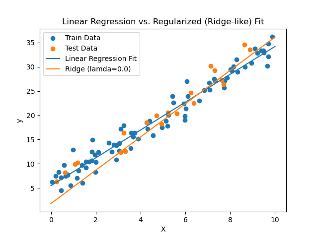
Figure 1: This caption has one line so it is centered

5. Conclusion

This study builds upon standard linear regression, addressing its limitations in noisy data prediction by proposing a regression method based on regularized hyperparameter optimization. By combining the normal equation with gradient descent, we enhance the model’s ability to capture data relationships, enabling it to robustly handle noise interference while achieving dynamic optimization through hyperparameter tuning. Additionally, we introduce a staged parameter estimation strategy to improve prediction accuracy and generalization performance. Experimental results show that standard linear regression achieves a mean squared error (MSE) of 3.90 on the test set, while our method optimizes the test MSE to 6.56 (at \( λ=0.0 \) ). Although it does not significantly outperform the baseline on the current dataset scale, it demonstrates potential in noise resistance. Despite progress in multiple areas, this study leaves room for further exploration. In the future, we plan to refine the convergence strategy of gradient descent to reduce training error and enhance regularized regression performance on small datasets. For example, an adaptive learning rate mechanism [14] tailored to data characteristics could accelerate parameter optimization. Additionally, we aim to test larger-scale simulated or real-world datasets to validate the method’s applicability in high-dimensional scenarios. Integrating regularization techniques like Lasso or Elastic Net [15] could further improve adaptability to feature selection. In practical applications, we envision deploying this method in dynamic predictive tasks, such as financial time series analysis or sensor data processing. Overall, this research not only effectively improves linear regression but also provides fresh insights for hyperparameter optimization-based model design, advancing regression methods in complex scenarios.

References

[1]. Su X, Yan X, Tsai C L. Linear regression[J]. Wiley Interdisciplinary Reviews: Computational Statistics, 2012, 4(3): 275-294.
[2]. Hoel P G. On methods of solving normal equations[J]. The Annals of Mathematical Statistics, 1941, 12(3): 354-359.
[3]. Lanczos C. Evaluation of noisy data[J]. Journal of the Society for Industrial and Applied Mathematics, Series B: Numerical Analysis, 1964, 1(1): 76-85.
[4]. Köksoy O. Multiresponse robust design: Mean square error (MSE) criterion[J]. Applied Mathematics and Computation, 2006, 175(2): 1716-1729.
[5]. Ying X. An overview of overfitting and its solutions[C]//Journal of physics: Conference series. IOP Publishing, 2019, 1168: 022022.
[6]. Ramsay J, Hooker G. Dynamic data analysis[J]. Springer New York, New York, NY. doi, 2017, 10: 978-1.
[7]. McDonald G C. Ridge regression[J]. Wiley Interdisciplinary Reviews: Computational Statistics, 2009, 1(1): 93-100.
[8]. Ruder S. An overview of gradient descent optimization algorithms[J]. arXiv preprint arXiv:1609.04747, 2016.
[9]. Goeman J, Meijer R, Chaturvedi N. L1 and L2 penalized regression models[J]. cran. r-project. or, 2012.
[10]. Solli-Sæther H, Gottschalk P. The modeling process for stage models[J]. Journal of Organizational Computing and Electronic Commerce, 2010, 20(3): 279-293.
[11]. Denenberg J N. Anti-noise[J]. IEEE potentials, 1992, 11(2): 36-40.
[12]. Seeger M W. Cross-Validation Optimization for Large Scale Structured Classification Kernel Methods[J]. Journal of Machine Learning Research, 2008, 9(6).
[13]. Adami C. What is complexity?[J]. BioEssays, 2002, 24(12): 1085-1094.
[14]. Zeiler M D. Adadelta: an adaptive learning rate method[J]. arXiv preprint arXiv:1212.5701, 2012.
[15]. Schmidt M, Fung G, Rosales R. Fast optimization methods for l1 regularization: A comparative study and two new approaches[C]//Machine Learning: ECML 2007: 18th European Conference on Machine Learning, Warsaw, Poland, September 17-21, 2007. Proceedings 18. Springer Berlin Heidelberg, 2007: 286-297.
Cite this article
Li,W. (2025). Linear Regression with Regularized Hyperparameter Optimization. Theoretical and Natural Science,105,106-112.
Data availability
The datasets used and/or analyzed during the current study will be available from the authors upon reasonable request.
Disclaimer/Publisher's Note
The statements, opinions and data contained in all publications are solely those of the individual author(s) and contributor(s) and not of EWA Publishing and/or the editor(s). EWA Publishing and/or the editor(s) disclaim responsibility for any injury to people or property resulting from any ideas, methods, instructions or products referred to in the content.
About volume
Volume title: Proceedings of the 3rd International Conference on Mathematical Physics and Computational Simulation
© 2024 by the author(s). Licensee EWA Publishing, Oxford, UK. This article is an open access article distributed under the terms and
conditions of the Creative Commons Attribution (CC BY) license. Authors who
publish this series agree to the following terms:
1. Authors retain copyright and grant the series right of first publication with the work simultaneously licensed under a Creative Commons
Attribution License that allows others to share the work with an acknowledgment of the work's authorship and initial publication in this
series.
2. Authors are able to enter into separate, additional contractual arrangements for the non-exclusive distribution of the series's published
version of the work (e.g., post it to an institutional repository or publish it in a book), with an acknowledgment of its initial
publication in this series.
3. Authors are permitted and encouraged to post their work online (e.g., in institutional repositories or on their website) prior to and
during the submission process, as it can lead to productive exchanges, as well as earlier and greater citation of published work (See
Open access policy for details).