1. Introduction

With the rapid development of drone and small aircraft technology, the low-altitude economy has gradually become a hot topic. The low-altitude economy is an economic form derived from the low-altitude flight activities of civil manned or unmanned aircraft, encompassing aircraft research and development, manufacturing, commercial operations, and infrastructure construction.

The rapid development of the low-altitude economy and the significant relaxation of regulations in low-altitude airspace have provided aircraft with greater operational space, while also posing significant challenges to the planning and regulation of low-altitude airspace. Airspace management not only involves technical details such as the flight paths and altitudes of aircraft but also requires consideration of multiple dimensions including safety, efficiency, and environmental protection.

Low-altitude airspace planning encompasses multiple aspects: grid technology, remote sensing, communication and networking, aircraft route planning, and operational management [1]. This study primarily focuses on the construction of geofencing technology and airspace stratification technology within the airspace structure, specially the conflict resolution problem between spatiotemporal conflict airspace requirements. Although this technology segments the airspace and reduces its utilization efficiency, it offers unparalleled advantage of safety [2].

Generally, aircraft users submit airspace usage requests to the control center, which include the horizontal position area, the altitude range of the airspace, and the time range for usage. When two airspace applications are in conflict simultaneously in terms of time, altitude, and horizontal range, it is considered an airspace conflict. Specifically, this situation occurs when there is an overlap in all three dimensions of the airspace or when the distances between the ranges are less than the safety intervals.

Due to the large number of users, it is necessary to adjust conflicting user demands and optimize airspace resource allocation in order to maximize user needs and utilize airspace resources more effectively. The airspace applications in conflict are shown in Figure 1.

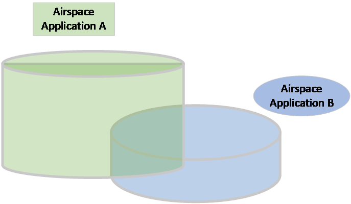
Figure 1: Airspace applications are in conflict

2. Literature review

Since the 1940s, researchers have conducted extensive studies on various issues in the field of airspace planning, leading to a plethora of algorithms and models. Numerous scholars have focused on airspace conflict detection and resolution planning based on aircraft trajectories and spatial grid partitioning systems.

Kuchar et al. [3] conducted a review of aircraft dynamic trajectory prediction, conflict detection, and resolution techniques since 2000, investigating 68 modeling methods for conflict detection and resolution. They classified and evaluated these methods based on the dimensions of state information, dynamic propagation methods, conflict detection thresholds, conflict resolution methods, maneuvering sizes and so on.

Pallottino et al. [4] studied the issue of conflicts between aircrafts flying in shared airspace. They established mixed-integer linear programming models for two scenarios: one allowing only changes in speed and the other allowing only changes in heading angle, and employed solvers to address the problem.

Ayuso et al. [5] proposed a hybrid 0-1 linear optimization model based on geometric transformations for airspace conflict detection and resolution. Knowing the initial coordinates, directional angles, and flight altitudes, conflict resolution is achieved by minimizing several objective functions (such as the variation in each dimension and the number of dimensions that changed) while enforcing a return to the original flight configuration in the absence of aircraft conflicts.

Tang et al. [6] developed a conflict detection and resolution algorithm for small fixed-wing aircraft based on a Spatial Grid Partitioning System (SGPS). This algorithm determines whether two trajectories pass through the same grid space within an overlapping time window. They also proposed techniques based on time scheduling and vertical adjustment to achieve conflict resolution.

Miao et al. [7] proposed a low-altitude flight conflict detection algorithm based on a multi-level grid spatiotemporal index. This algorithm transforms the traditional conflict computation based on trajectory traversal into a grid conflict state query within a distributed grid database. The algorithm first constructs a spatiotemporal coding model based on airspace, then uses grid coding to identify trajectories and no-fly zones, and subsequently establishes a multi-level grid spatiotemporal index according to the table structure of the grid database. Finally, the algorithm designs an optimized query method to detect conflicts within the grid database.

These studies, in conducting airspace conflict detection and resolution, not only involve adjustments to the horizontal and vertical dimensions of the airspace but also include planning for the aircraft's heading and speed.

Due to the inherent non-linear nature of airspace conflict issues, it is difficult to establish a linear model, which increases the complexity of the solution. Some studies have linearized the non-linear problems to reduce the difficulty and directly applied solvers for resolution, while others have designed heuristic functions for solving. Tamas et al. [8] analyzed a lot of researches on the application of mixed-integer nonlinear optimization methods to air traffic management issues. They established a mixed-integer nonlinear model addressing airspace conflicts and resolution problems, and solved the model using a MINLP solver. They also examined the application of heuristic methods such as Branch and Bound, linearization methods, and neighborhood search in problem-solving.

3. Mathematical programming model

This study addresses the problem of airspace conflict detection and resolution by constructing a mixed-integer linear model. The conflict resolution is achieved through adjustments in the horizontal, vertical, and temporal dimensions. Different dimensions have different priorities, while minimizing adjustments to user applications and rejecting requests as little as possible. And solutions are obtained using a solver.

3.1. Notations

The symbols used in the model of this article are explained as follows:

Table 1: Parameters definition

Table 2: Variables definition

3.2. Equations

Based on the above symbol description, a mixed-integer nonlinear programming model is constructed for the low-altitude airspace planning problem as follows:

\( min  p1*rejectnum+p2*Adjustnum+p3*T+p4*S \) (1)

S.t.

\( {p_{i,d}}+{x_{i,d}} \gt bmi{n_{d}}+p{r_{i,d}} \) (2)

\( {p_{i,d}}+{x_{i,d}} \lt bma{x_{d}}-p{r_{i,d}} \) (3)

\( |{x_{i,d}}| \lt {δ_{d}} \) (4)

\( (1-bool(|{p_{i,1}}+{x_{i,1}}-{p_{j,1}}-{x_{j,1}}| \gt {λ_{1}}+p{r_{i,1}}+p{r_{j,1}}))* \)

\( (1-bool(|{p_{i,2}}+{x_{i,2}}-{p_{j,2}}-{x_{j,2}}| \gt {λ_{2}}+p{r_{i,2}}+p{r_{j,2}}))* \) (5)

\( (1-bool(temp \gt {λ_{3}}+p{r_{i,3}}+p{r_{j,3}}))=0 \)

\( |({p_{i,3}}+{x_{i,3}},{p_{i,4}}+{x_{i,4}})-({p_{j,3}}+{x_{j,3}},{p_{j,4}}+{x_{j,4}})|=temp \) (6)

\( {x_{i.d}}-dplu{s_{i.d}}+dmin{i_{i.d}}=0 \) (7)

\( dрlu{s_{i,d}} \lt {δ_{d}}+{z_{i}}*M \) (8)

\( d{тіпі_{i,d}} \lt {δ_{d}}+{z_{i}}*M \) (9)

\( dplu{s_{id}} \lt {y_{i}}*M \) (10)

\( d{тіпі_{i,d}} \lt {y_{i}}*M \) (11)

\( T=\sum _{i∈N} dplu{s_{i,1}}+dmin{i_{i,1}} \) (12)

\( S=\sum _{i∈N}^{d=2..4} dplu{s_{i,d}}+dmin{i_{i,d}} \) (13)

Equation (2) and Equation (3) represent the marginal constraint. Equation (4) represents the constraint on the maximum adjustment amount. Equation (5) and Equation (6) indicates that there is no conflict between the airspace demands. Equation (7), Equation (8), Equation (9), Equation (10), Equation (11), Equation (12) and Equation (13) represent the relationship between variables.

4. Linearization

Clearly, the model has multiple nonlinear constraints. Therefore, it is considered to linearize the model and transform it into a mixed-integer quadratic programming model.

4.1. Multidimensional boolean product linearization

Introducing infinitesimals and Boolean variables into the variables to achieve the decomposition of equation (5).

\( |{p_{i,2}}+{x_{i,2}}-{p_{j,2}}-{x_{j,2}}|+M*hboo{l_{i,j}} \gt {λ_{2}}+p{r_{i,2}}+p{r_{j,2}} \) (14)

\( |{p_{i,1}}+{x_{i,1}}-{p_{j,1}}-{x_{j,1}}|+M*tboo{l_{i,j}} \gt {λ_{1}}+p{r_{i,1}}+p{r_{j,1}} \) (15)

\( temp \gt {λ_{1}}+p{r_{i,1}}+p{r_{j,1}}+(tboo{l_{i,j}}-1)*M+(hboo{l_{i,j}}-1)*M \) (16)

Proof.

\( |{p_{i,2}}+{x_{i,2}}-{p_{j,2}}-{x_{j,2}}| \gt {λ_{2}}+p{r_{i,2}}+p{r_{j,2}}⇒hboo{l_{i,j}}=\lbrace 0,1\rbrace \) (17)

\( |{p_{i,2}}+{x_{i,2}}-{p_{j,2}}-{x_{j,2}}| \lt {λ_{2}}+p{r_{i,2}}+p{r_{j,2}}⇒hboo{l_{i,j}}=1 \) (18)

\( minhboo{l_{i,j}}|{p_{i,2}}+{x_{i,2}}-{p_{j,2}}-{x_{j,2}}| \gt {λ_{2}}+p{r_{i,2}}+p{r_{j,2}}⇒hboo{l_{i,j}}=0 \) (19)

\( |{p_{i,1}}+{x_{i,1}}-{p_{j,1}}-{x_{j,1}}| \gt {λ_{1}}+p{r_{i,1}}+p{r_{j,1}}⇒tboo{l_{i,j}}=\lbrace 0,1\rbrace \) (20)

\( |{p_{i,1}}+{x_{i,1}}-{p_{j,1}}-{x_{j,1}}| \lt {λ_{1}}+p{r_{i,1}}+p{r_{j,1}}⇒tboo{l_{i,j}}=1 \) (21)

\( mintboo{l_{i,j}}|{p_{i,1}}+{x_{i,1}}-{p_{j,1}}-{x_{j,1}}| \gt {λ_{1}}+p{r_{i,1}}+p{r_{j,1}}⇒tboo{l_{i,j}}=0 \) (22)

if \( tboo{l_{i,j}}=0 \) or \( hboo{l_{i,j}}=0 \) , then \( |{p_{i,1}}+{x_{i,1}}-{p_{j,1}}-{x_{j,1}}| \gt {λ_{1}}+p{r_{i,1}}+p{r_{j,1}}-M \) .if \( tboo{l_{i,j}}=1 \) and \( hboo{l_{i,j}}=1 \) , then \( |{p_{i,1}}+{x_{i,1}}-{p_{j,1}}-{x_{j,1}}| \gt {λ_{1}}+p{r_{i,1}}+p{r_{j,1}} \) .

This method allows for the decomposition of equation (5) without altering the meaning of the constraints in it.

4.2. Quadratic function linearization

The linearization of the distance (squared term) between two points can be achieved by introducing an intermediate variable, which can transform the point information of that distance into interval information. Although this may introduce some bias in the precise solution of the model, it allows for the linearization of the constraints, effectively reducing the problem space.Sentence (6) can be linearized in this way.

\( tem{p^{2}}={({p_{i,3}}+{x_{i,3}}-{p_{j,3}}+{x_{j,3}})^{2}}+{({p_{i,4}}+{x_{i,4}}-{p_{j,4}}+{x_{j,4}})^{2}} \) (23)

\( tem{p^{2}} \gt 2*min(|{p_{i,3}}+{x_{i,3}}-{p_{j,3}}+{x_{j,3}}|)*|{p_{i,3}}+{x_{i,3}}-{p_{j,3}}+{x_{j,3}}| \)

\( -min(|{p_{i,3}}+{x_{i,3}}-{p_{j,3}}+{x_{j,3}}|{)^{2}}+2*min(|{p_{i,4}}+{x_{i,4}}-{p_{j,4}}+{x_{j,4}}|) \) (24)

\( *|{p_{i,4}}+{x_{i,4}}-{p_{j,4}}+{x_{j,4}}|-min(|{p_{i,4}}+{x_{i,4}}-{p_{j,4}}+{x_{j,4}}|{)^{2}} \)

\( tem{p^{2}} \gt 2*max(|{p_{i,3}}+{x_{i,3}}-{p_{j,3}}+{x_{j,3}}|)*|{p_{i,3}}+{x_{i,3}}-{p_{j,3}}+{x_{j,3}}| \)

\( -max(|{p_{i,3}}+{x_{i,3}}-{p_{j,3}}+{x_{j,3}}|{)^{2}}+2*max(|{p_{i,4}}+{x_{i,4}}-{p_{j,4}}+{x_{j,4}}|) \) (25)

\( *|{p_{i,4}}+{x_{i,4}}-{p_{j,4}}+{x_{j,4}}|-max(|{p_{i,4}}+{x_{i,4}}-{p_{j,4}}+{x_{j,4}}|{)^{2}} \)

Proof.

If \( c∈[a,b] \) , then \( {c^{2}} \gt {a^{2}}+2a*(c-a)=2ac-{a^{2}} \) , \( {b^{2}} \gt {c^{2}}+2c*(b-c)=2bc-{c^{2}} \) .

Since the constraint on \( temp \) is greater than a certain value, \( temp \) can be replaced by the right-hand side of the equation (18) and equation (19).

Obviously, \( max{(|{p_{i,3}}+{x_{i,3}}-{p_{j,3}}-{x_{j,3}}|)}=|{p_{i,3}}-{p_{j,3}}|-2*{δ_{3}} \) , \( min{(|{p_{i,3}}+{x_{i,3}}-{p_{j,3}}-{x_{j,3}}|)}=|{p_{i,3}}-{p_{j,3}}|+2*{δ_{3}} \) , \( max{(|{p_{i,4}}+{x_{i,4}}-{p_{j,4}}-{x_{j,4}}|)}=|{p_{i,4}}-{p_{j,4}}|-2*{δ_{4}} \) , \( min{(|{p_{i,4}}+{x_{i,4}}-{p_{j,4}}-{x_{j,4}}|)}=|{p_{i,4}}-{p_{j,4}}|+2*{δ_{4}} \) .

4.3. Absolute value linearization

For absolute value constraints, they can be implemented by adding a big M and Boolean variables to the model.

\( tempboo{l_{i,j,d}}*M+{p_{i,d}}+{x_{i,d}}-{p_{j,d}}-{x_{j,d}} \gt 0 \) (26)

\( mintempboo{l_{i,j,d}} \) (27)

Add \( tempbool * M \) to the right side of the inequalities, and in this way, the absolute value constraints will be linearized.

4.4. Auxiliary variable constraints

After linearization, the objective can be represented as \( p1*rejectnum+p2*Adjustnum+p3*T+p4*S+tempboo{l_{i,j,d}}+dplu{s_{i,d}}+dmin{i_{i,d}} \) .

The Boolean variables introduced are defined in relation to two objects, and the relationship between these two is relative; it can be described using \( (i,j) \) as well as \( (j,i) \) . Based on the above characteristics, for each Boolean variable, add \( tempboo{l_{i,j,d}}+tempboo{l_{j,i,d}}=1 \) , \( tboo{l_{i,j}}+tboo{l_{j,i}}=1 \) and \( hboo{l_{i,j}}+hboo{l_{j,i}}=1 \) . In this way, the sum of these Boolean variables can be effectively restricted to a fixed value without affecting the objective function.

Through the above processing methods, the original nonlinear model can be linearized, and the linearized model can be directly incorporated into the processor for solving.

5. Numerical experiments and results

The experiment was implemented using CPLEX 12.9 Studio, and all experiments were run on a computer with an AMD Ryzen Threadripper PRO 5975WX 32-Cores 3.60 GHz processor, 32.0 GB (31.8 GB available) of memory, and the operating system Windows 10.

The data is described in Table 3.

Table 3: Rules to format sections

The experiment employs nine datasets with different demand quantities.The results are shown in Table 4.

Table 4: Rules to format sections

As shown in Figure 2, due to the rapid increase in computational complexity of the problem with the growing number of demands, the solver's performance tends to deteriorate when the scale is larger. The time required to solve the problem increases exponentially with the size of the problem. When the problem size exceeds 60, the solver is unable to obtain the optimal solution within an acceptable time period. Moreover, as the problem size increases, the gap value of the feasible solutions obtained by the solver becomes larger.

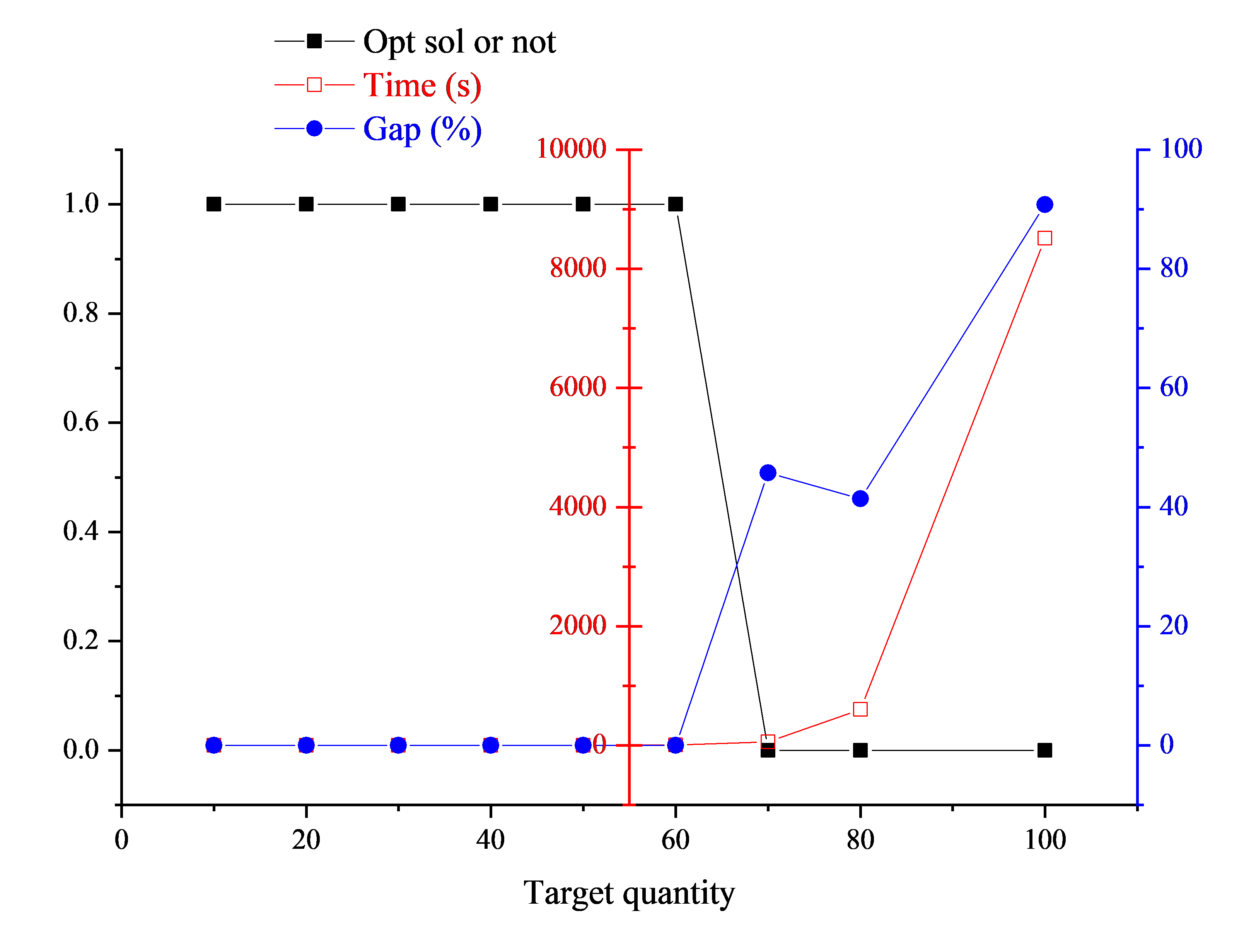
Figure 2: Line graph of experimental results

6. Conclusion

According to the linear estimation of the quadratic term: if \( c∈[a,b] \) , then \( {c^{2}} \gt {a^{2}}+2a*(c-a)=2ac-{a^{2}} \) , \( {b^{2}} \gt {c^{2}}+2c*(b-c)=2bc-{c^{2}} \) . The maximum degree of relaxation of this linearization method for the problem is \( \frac{{(a-b)^{2}}}{{(a+b)^{2}}} \) . For this question, the degree of relaxation is determined by the maximun and minimum distances between the two airspace demands. The error between the optimal solution of this linearization method and the optimal solution of the actual problem will also be controlled within this maximum relaxation level.

Specifically, for this problem, when \( max{(|{p_{i,3}}+{x_{i,3}}-{p_{j,3}}+{x_{j,3}}|)} \lt ({λ_{3}}+p{r_{i,3}}+p{r_{j,3}}) \) , the conflict cannot be resolved, and the relaxation of this constraint has no effect on the problem. When \( max{(|{p_{i,3}}+{x_{i,3}}-{p_{j,3}}+{x_{j,3}}|)} \gt ({λ_{3}}+p{r_{i,3}}+p{r_{j,3}}) \) , \( min{(|{p_{i,3}}+{x_{i,3}}-{p_{j,3}}+{x_{j,3}}|)} \gt ({λ_{3}}+p{r_{i,3}}+p{r_{j,3}}-4\sqrt[]{2}{δ_{3}}) \) , the degree of relaxation \( \frac{{(a-b)^{2}}}{{(a+b)^{2}}} \) will larger than \( \frac{{(4\sqrt[]{2}{δ_{3}})^{2}}}{{(2({λ_{3}}+p{r_{i,3}}+p{r_{j,3}})-4\sqrt[]{2}{δ_{3}})^{2}}} \) . As \( {δ_{3}}=10 \) and \( p{r_{i,3}}=100 \) , the small degree of relaxation has little impact on the problem.

In summary, the model proposed in this paper can be applied to the resolution of such problems. However, for large-scale problems, the solver's solving capability is not enough, necessitating more efficient algorithms.

References

[1]. Xu C., Liao X., & Yang F. (2022). Ieee standard pioneered an it-led interdisciplinary approach to structure low-altitude airspace for uav operations. Science China. Information Sciences, vol. 65,no. 10, p. 07201.
[2]. Vascik P. D., Hansman R. J. (2017). Evaluation of key operational constraints affecting on-demand mobility for aviation in the los angeles basin: ground infrastructure, air traffic control and noise. 17th AIAA Aviation Technology, Integration, and Operations Conference, p. 3084.
[3]. Kuchar J. K., Yang L. C. (2000). A review of conflict detection and resolution modeling methods. IEEE Transactions on intelligent transportation systems, vol. 1, no. 4, pp. 179–189.
[4]. Pallottino L., Feron E. M., & Bicchi A. (2002). Conflict resolution problems for air traffic management systems solved with mixed integer programming. IEEE transactions on intelligent trans-portation systems, vol. 3, no. 1, pp. 3–11.
[5]. Alonso-Ayuso A., Escudero L. F., & Martín-Campo F. J. (2010). Collision avoidance in air traffic management: A mixed-integer linear optimization approach. IEEE transactions on intelligent transportation systems, vol. 12, no. 1, pp. 47–57.
[6]. Tang J., Yang W. (2018). A causal model for safety assessment purposes in opening the low-altitude urban airspace of chinese pilot cities. Journal of Advanced Transportation, vol. 2018, no. 1, p. 5042961.
[7]. Miao S., Cheng C., Zhai W., Ren F., Zhang B., Li S., Zhang J. & Zhang H. (2019). A low-altitude flight conflict detection algo-rithm based on a multilevel grid spatiotemporal index. ISPRS International Journal of Geo-Information, vol. 8, no. 6, p. 289.
[8]. Wild S. (2017). Advances and trends in optimization with engineering applications.
Cite this article
Yu,G.;Lei,T.;Li,K.;Qiu,H.;Li,Y. (2025). Research on the Application of Linearization Model Methods in Low Altitude Airspace Planning. Theoretical and Natural Science,109,42-49.
Data availability
The datasets used and/or analyzed during the current study will be available from the authors upon reasonable request.
Disclaimer/Publisher's Note
The statements, opinions and data contained in all publications are solely those of the individual author(s) and contributor(s) and not of EWA Publishing and/or the editor(s). EWA Publishing and/or the editor(s) disclaim responsibility for any injury to people or property resulting from any ideas, methods, instructions or products referred to in the content.
About volume
Volume title: Proceedings of CONF-MPCS 2025 Symposium: Leveraging EVs and Machine Learning for Sustainable Energy Demand Management
© 2024 by the author(s). Licensee EWA Publishing, Oxford, UK. This article is an open access article distributed under the terms and
conditions of the Creative Commons Attribution (CC BY) license. Authors who
publish this series agree to the following terms:
1. Authors retain copyright and grant the series right of first publication with the work simultaneously licensed under a Creative Commons
Attribution License that allows others to share the work with an acknowledgment of the work's authorship and initial publication in this
series.
2. Authors are able to enter into separate, additional contractual arrangements for the non-exclusive distribution of the series's published
version of the work (e.g., post it to an institutional repository or publish it in a book), with an acknowledgment of its initial
publication in this series.
3. Authors are permitted and encouraged to post their work online (e.g., in institutional repositories or on their website) prior to and
during the submission process, as it can lead to productive exchanges, as well as earlier and greater citation of published work (See
Open access policy for details).